Spatial Patterns

How to discover and to describe

Chris Reudenbach

Spatial Patterns

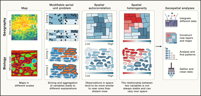
Discovering and describing spatial patterns is an important part of many geographical studies, and spatial patterns are linked to natural and social processes.

Corona Virus Distribution, https://coronavirus.jhu.edu/map.html

Spatial patterns of categorical raster data

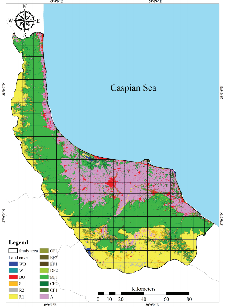
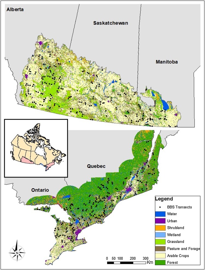
Numerous geographical studies are linked to all kind of classified raster based spatial data

https://doi.org/10.1016/j.agee.2020.107052

Types of spatial patterns

Point patterns versus continous patterns

Point Distributions, (https://gisgeography.com/spatial-patterns

Raster based patterns, Source: https://www.cell.com/cell/fulltext/S0092-8674%2823%2901219-9

Dynamics of spatial patterns

Dynamic evaluation of landscape transformations, https://www.landscape-online.org/index.php/lo/article/view/LO.2022.1097/LO.2022.1097

Quantification of categorical spatial patterns

Spatial patterns can be quantified using landscape metrics (O’Neill et al. 1988; Turner and Gardner 1991; Li and Reynolds 1993; He et al. 2000; Jaeger 2000; Kot i in. 2006; McGarigal 2014).

Software such as FRAGSTATS, GuidosToolbox, or landscapemetrics has proven useful in many scientific studies (> 12,000 citations).

There is a relationship between an area’s pattern composition and configuration and ecosystem characteristics, such as vegetation diversity, animal distributions, and water quality within this area (Hunsaker i Levine, 1995; Fahrig i Nuttle, 2005; Klingbeil i Willig, 2009; Holzschuh et al., 2010; Fahrig et al., 2011; Carrara et al., 2015; Arroyo-Rodŕıguez et al. 2016; Duflot et al., 2017, many others..)

Example data

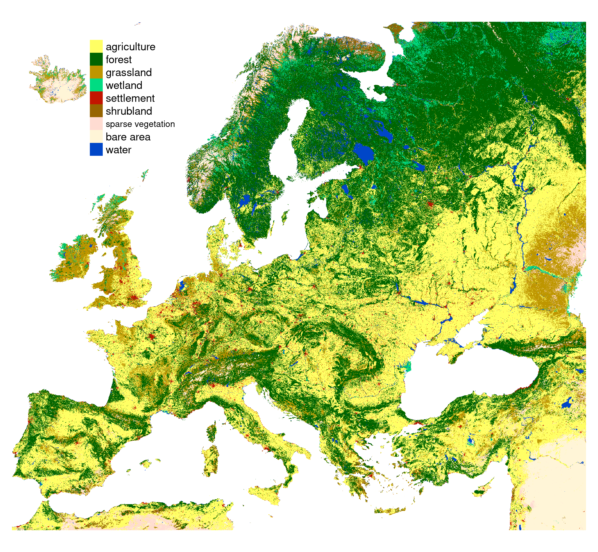
Land cover data for the year 2016 from the CCI-LC project
Simplified into nine main categories
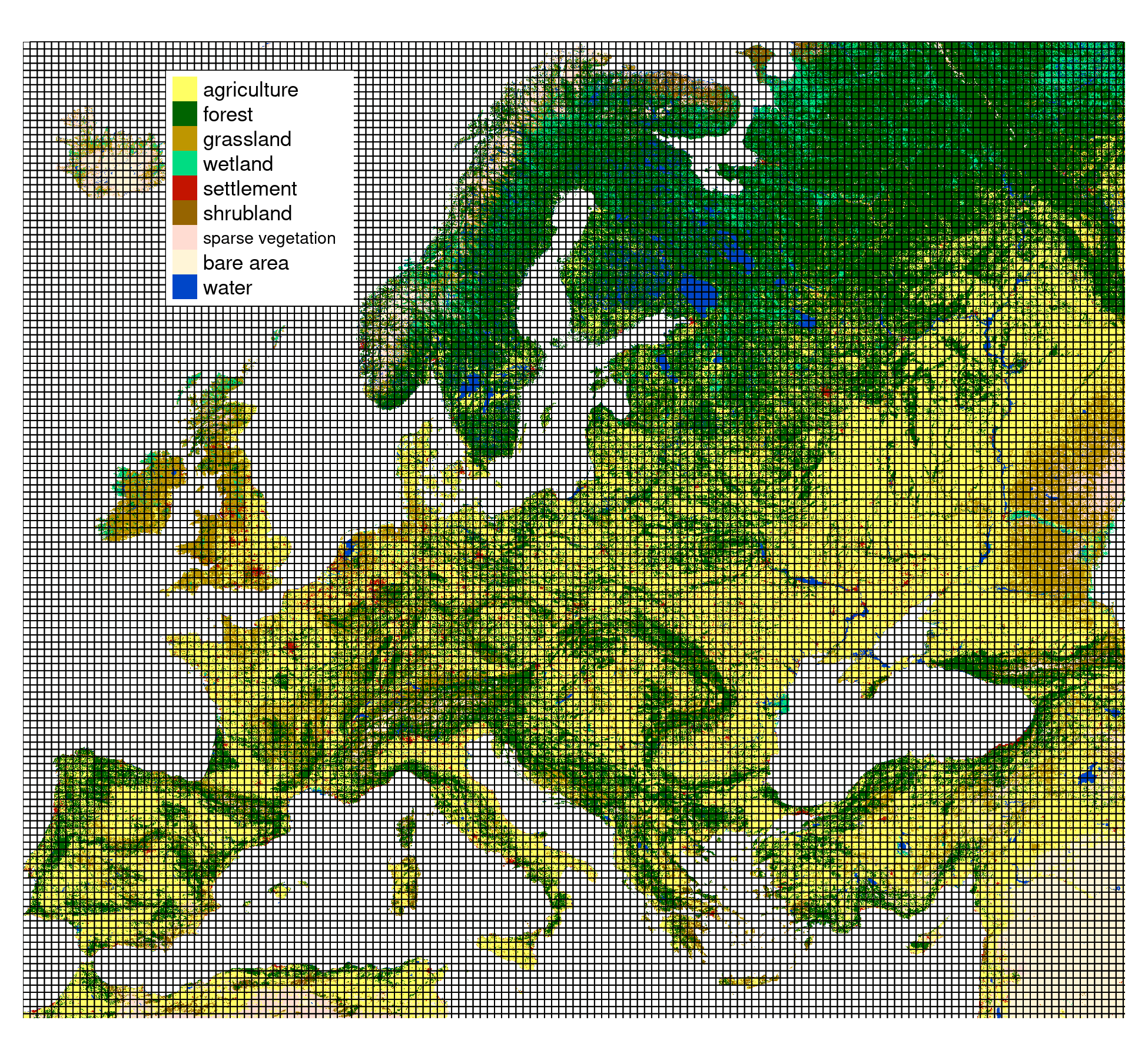
Partitioned into 30 x 30 kilometers square blocks
13,909 categorical rasters (100x100 cells) https://agupubs.onlinelibrary.wiley.com/doi/epdf/10.1029/2020JD033031

—

Example Data

Randomely selected 16 rasters with different proportions of forest (green) areas:

Landscape Metrics

In the last 40 or so years, several hundred different landscape metrics were developed
They quantify the composition and configuration of spatial patterns of categorical rasters
General assumption is that the spatial pattern of a landscape influences the processes that occur within it
Landscape metrics can be calculated for three different levels: patch, class, and landscape (here we focus on the landscape level)
They can be divided into several groups: (1) area and edge metrics, (2) shape metrics, (3) core metrics, (4) aggregation metrics, (5) diversity metrics, (6) complexity metrics

Landscape Metrics

Important considerations:

Scale: the size of the area over which the metrics are calculated
Extent: the borders of the study area
Spatial resolution: the size of the raster cells
Categorization: the categories used in the analysis
Redundancy: many metrics are highly correlated

Landscape Metrics

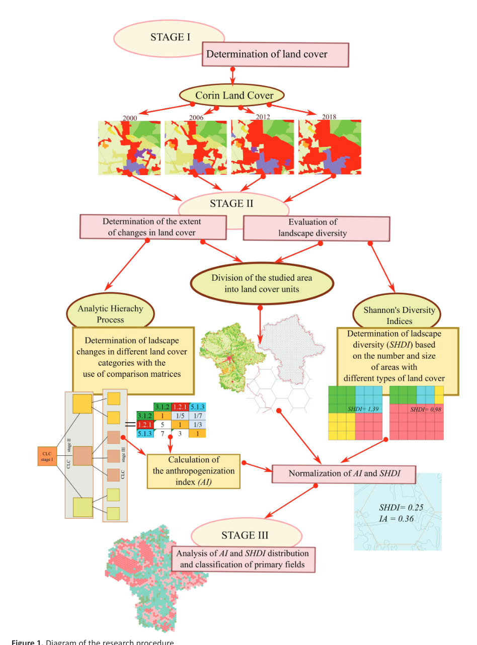
SHDI - Shannon’s diversity index - takes both the number of classes and the abundance of each class into account; larger values indicate higher diversity

AI - Aggregation index - from 0 for maximally disaggregated to 100 for maximally aggregated classes

Code examples

Taken from : “The landscapemetrics and motif packages for measuring landscape patterns and processes”

Read and visualize the data

library(landscapemetrics)
library(terra)
r9 = rast("exdata/r9.tif")
r1 = rast("exdata/r1.tif")
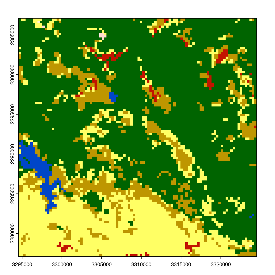
plot(r1); plot(r9)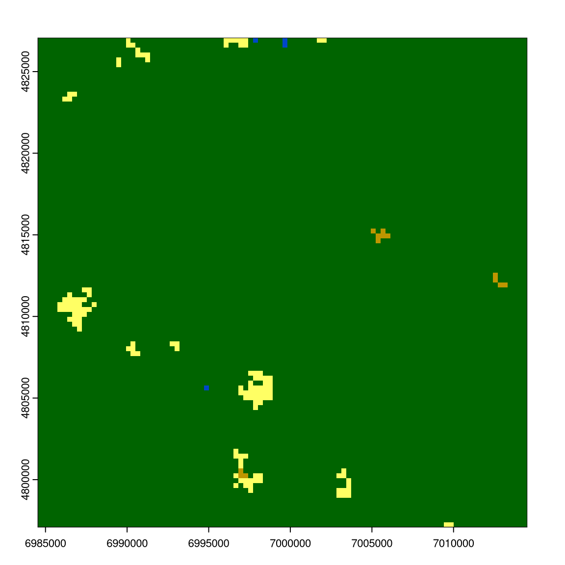

Get the indices

lsm_l_shdi(r9)

# A tibble: 1 × 6
  layer level     class    id metric value
  <int> <chr>     <int> <int> <chr>  <dbl>
1     1 landscape    NA    NA shdi    1.06

lsm_l_ai(r9)

# A tibble: 1 × 6
  layer level     class    id metric value
  <int> <chr>     <int> <int> <chr>  <dbl>
1     1 landscape    NA    NA ai      82.1

calculate_lsm(r9, what = c("lsm_l_shdi", "lsm_l_ai"))

# A tibble: 2 × 6
  layer level     class    id metric value
  <int> <chr>     <int> <int> <chr>  <dbl>
1     1 landscape    NA    NA ai     82.1 
2     1 landscape    NA    NA shdi    1.06

two_r = list(r1, r9)
calculate_lsm(two_r, what = c("lsm_l_shdi", "lsm_l_ai"))

# A tibble: 4 × 6
  layer level     class    id metric   value
  <int> <chr>     <int> <int> <chr>    <dbl>
1     1 landscape    NA    NA ai     98.7   
2     1 landscape    NA    NA shdi    0.0811
3     2 landscape    NA    NA ai     82.1   
4     2 landscape    NA    NA shdi    1.06

Code examples

mat_window = matrix(1, nrow = 11, ncol = 11)
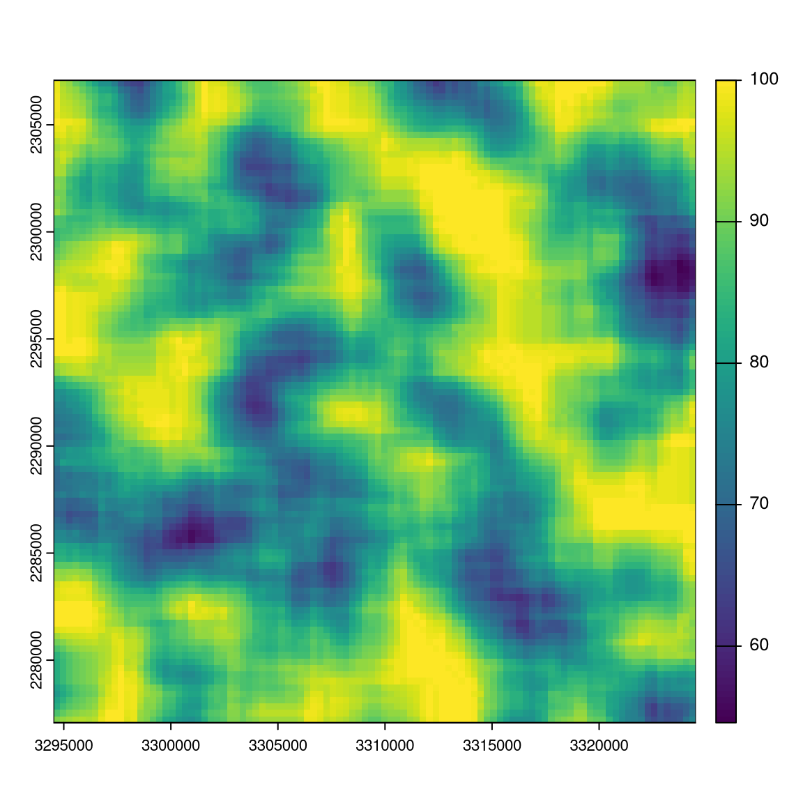
w_result = window_lsm(r9, window = mat_window, what = "lsm_l_ai")
plot(r9); plot(w_result$layer_1$lsm_l_ai)

Package landscapemetrics

https://r-spatialecology.github.io/landscapemetrics/

# A tibble: 133 × 5
   metric name                                type           level function_name
   <chr>  <chr>                               <chr>          <chr> <chr>        
 1 area   patch area                          area and edge… patch lsm_p_area   
 2 cai    core area index                     core area met… patch lsm_p_cai    
 3 circle related circumscribing circle       shape metric   patch lsm_p_circle 
 4 contig contiguity index                    shape metric   patch lsm_p_contig 
 5 core   core area                           core area met… patch lsm_p_core   
# ℹ 134 more rows

Sampling around points of interest
Moving window calculations
Calculating landscape metrics for irregular areas
Visualizations
More…

Exercises

Read the data from exdata/lc_small.tif and visualize it. What is the location of the data? What are the extent of the data and its spatial resolution? How many categories it contains?
Calculate Aggregation Index (AI) for the raster. Interpret the results.
Calculate Total Edge (TE) for the raster. Interpret the results. Next, read the data from `exdata/lc_small2.tif, calculate AI and TE for this raster, and compare the results with the previous raster.
Calculate Total Edge (TE) for the raster, but this time in a moving window of 9 by 9 cells. Visualize the results.
(Extra) Using the read_sf() function from the sf package, read the exdata/points.gpkg file. Next, calculate SHDI and AI of an area of 3000 meters from each sampling point (see the sample_lsm() function).