Landscape Patterns

How to discover and to describe

Chris Reudenbach

Landscape Metrics

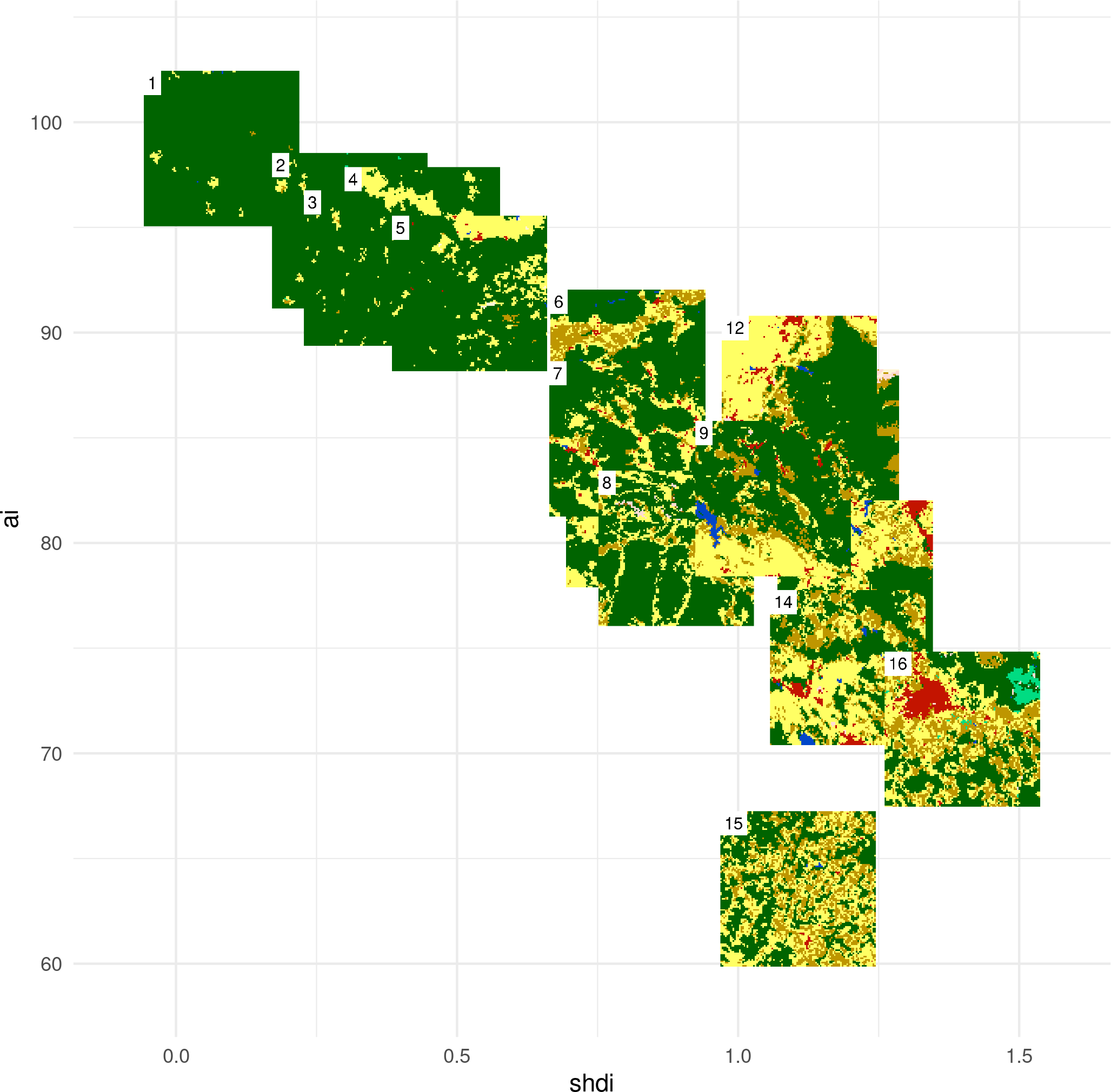
• Problem no. 1: which of the hundreds of spatial metrics should we choose?
• Problem no. 2: many landscape metrics are highly correlated…

Possible Approach - PCA of type samples of landscape metrics

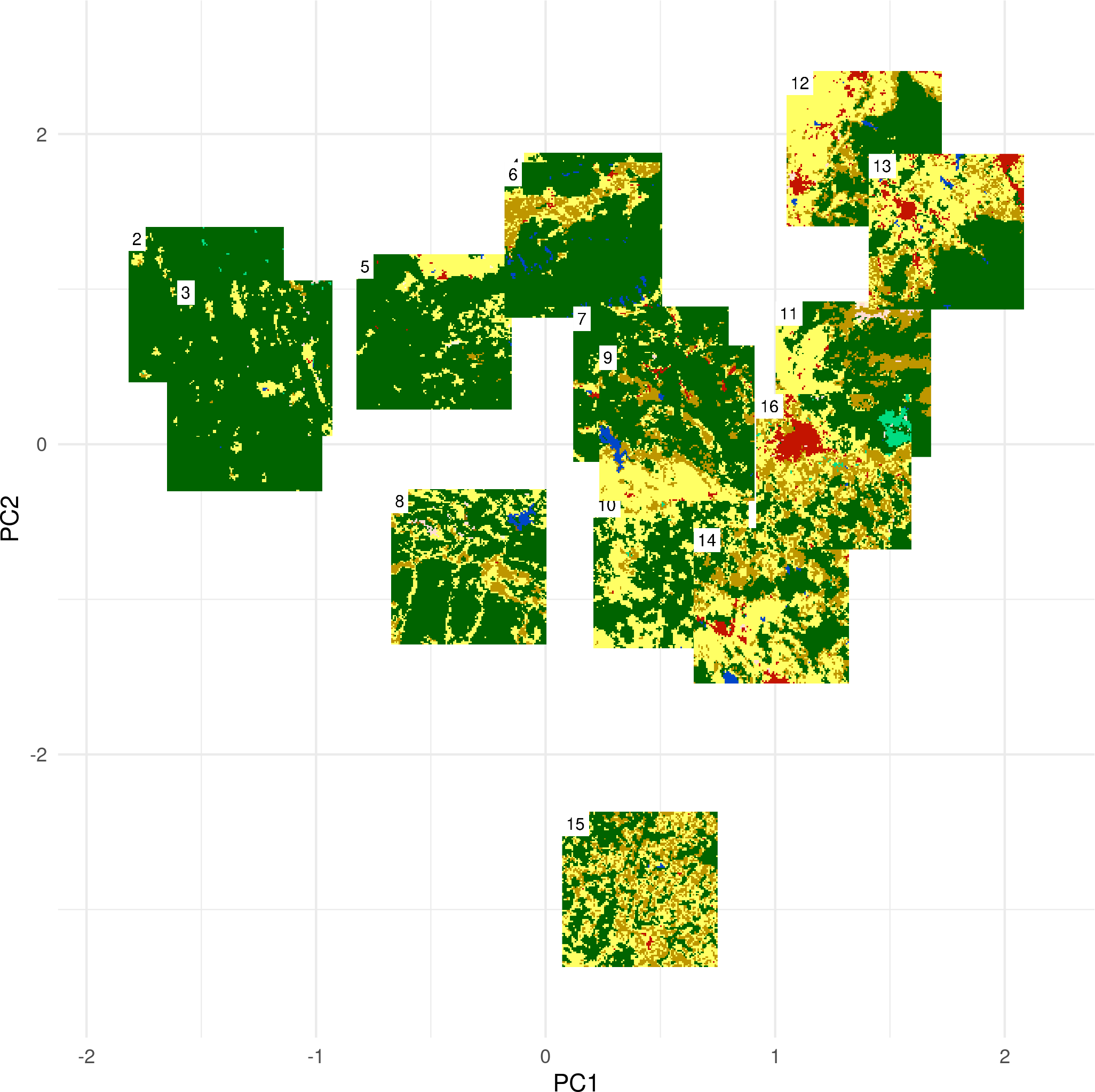
We performed a principal component analysis (PCA) using 17 landscape-level metrics:

PCA of landscape metrics

PCA 1

PCA 2

• First two principal components explained ~71% of variability

PCA of landscapes

The result allows to distinguish between:

• simple and complex rasters (left<->right)
• agmented and consolidated rasters (bottom<->top)

PCA 2

However, there are still some problems here…

PCA of landscapes

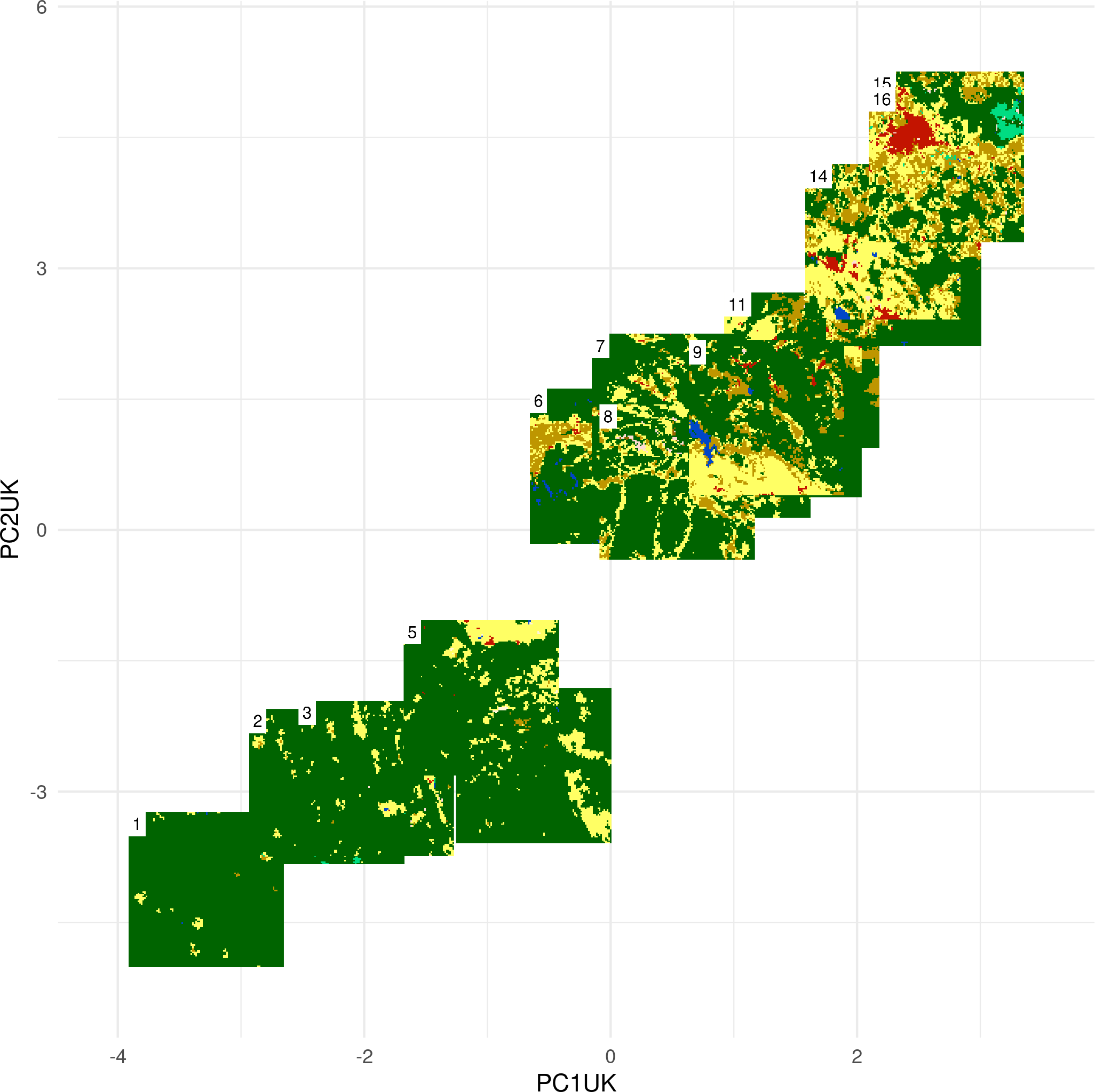
• We performed a second PCA using data from the United Kingdom only
• Next, we predicted the results on the data for the whole Europe

PCA 1

PCA 2

PCA of landscapes

PCA 1 PCA 2 UK EU

Issues with the PCA approach:

• Each new dataset requires recalculation of both, landscape metrics and principal components analysis (PCA)
• Highly correlated landscape metrics are used
• PCA results interpretation is not straightforward

IT metrics

• Five information theory metrics based on a co-occurrence matrix exist (Nowosad and Stepinski, 2019, https://doi.org/10.1007/s10980-019-00830-x)
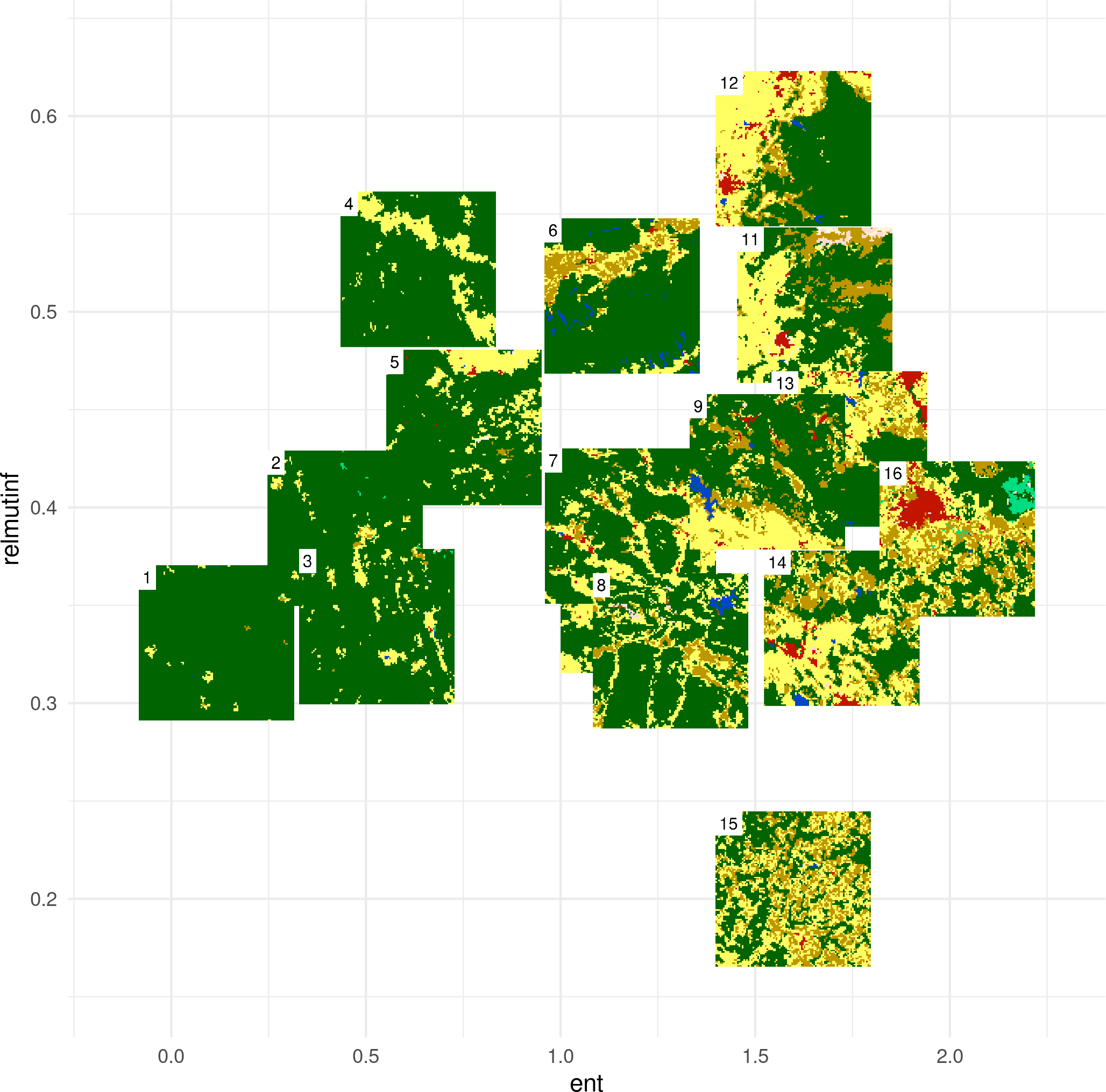
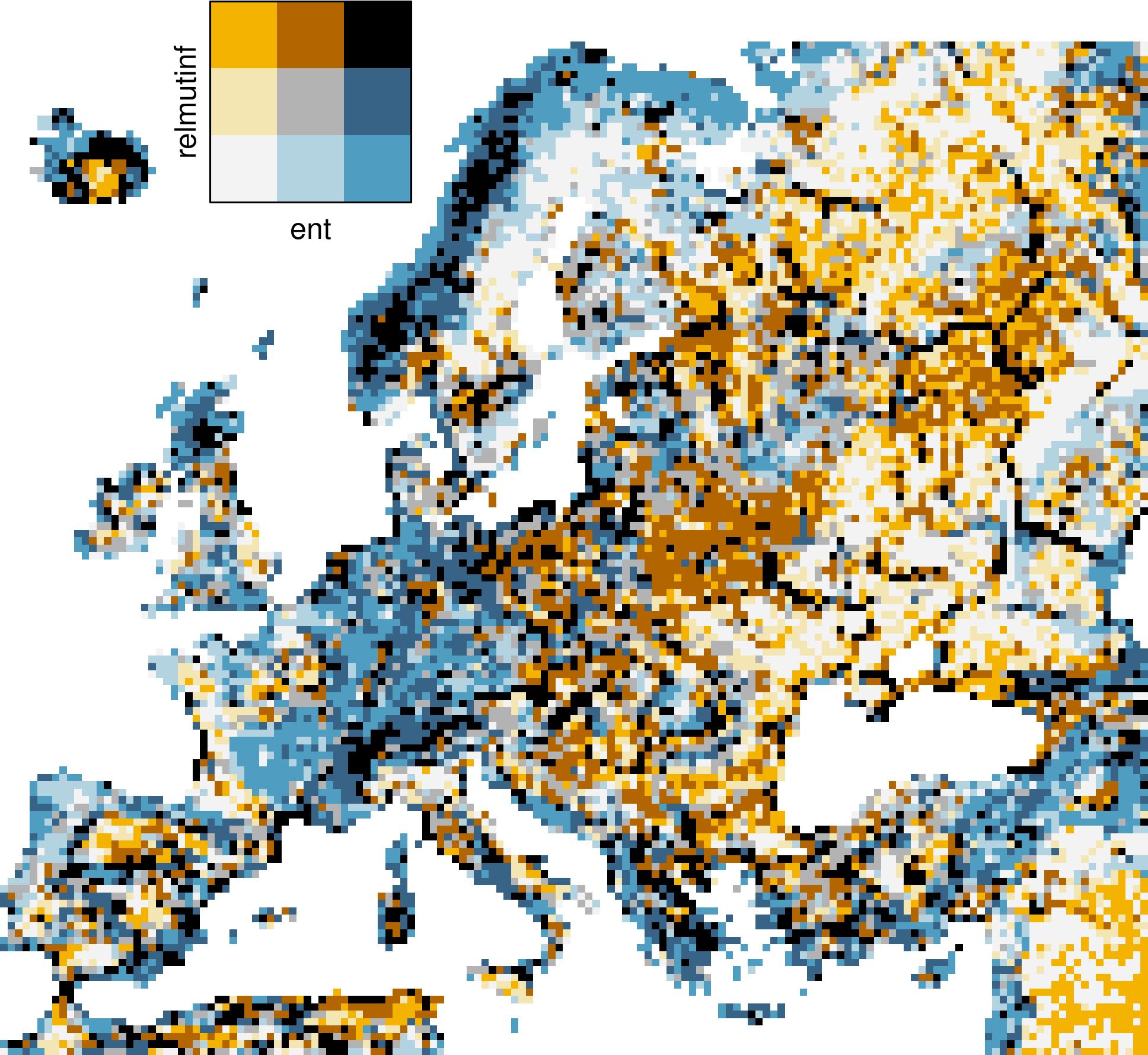
• Marginal entropy [H(x)] - diversity (composition) of spatial categories - from monothematic patterns to multithematic patterns
• Relative mutual information [U] - clumpiness (configuration) of spatial categories from fragmented patterns to consolidated patterns)
• H(x) and U are uncorrelated

Entropy

Relative mutual information

IT metrics

2D parametrization of categorical rasters’ configurations based on two weakly correlated IT metrics groups similar patterns into distinct regions of the parameters space

IT metrics final results

Land cover data

Parametrization of two IT metrics

Exercises

1. The marginal entropy and relative mutual information can be calculated using the landscapemetrics package’s functions: lsm_l_ent() and lsm_l_relmutinf(). Calculate both of these metrics for the exdata/lc_small.tif raster.
2. Read the exdata/lc_europe.tif raster using rast() from the **terra** package and theexdata/polygons.gpkgvector data using theread_sf()function from the **sf** package. Calculate the marginal entropy and relative mutual information for each polygon using thesample_lsm()` function.
3. Join the calculated values with the polygons (see https://r-spatialecology.github.io/landscapemetrics/articles/irregular_areas.html for more details).
4. Calculate SHDI and AI for the polygons. Compare the values of SHDI and AI with the marginal entropy and relative mutual information (e.g., using a scatterplot or by calculating the correlation coefficient). Are the results similar?
5. (Extra) Create your own polygonal grid using st_make_grid() function from the sf package for the area from the exdata/polygons.gpkg file. Calculate the marginal entropy and relative mutual information for each square using the sample_lsm() function. Visualize the results.

IT metrics

These metrics still leave some questions open…

• Relative mutual information is a result of dividing mutual information by entropy. What to do when the entropy is zero?
• How to incorporate the meaning of categories into the analysis?

Parametrization of two IT metrics

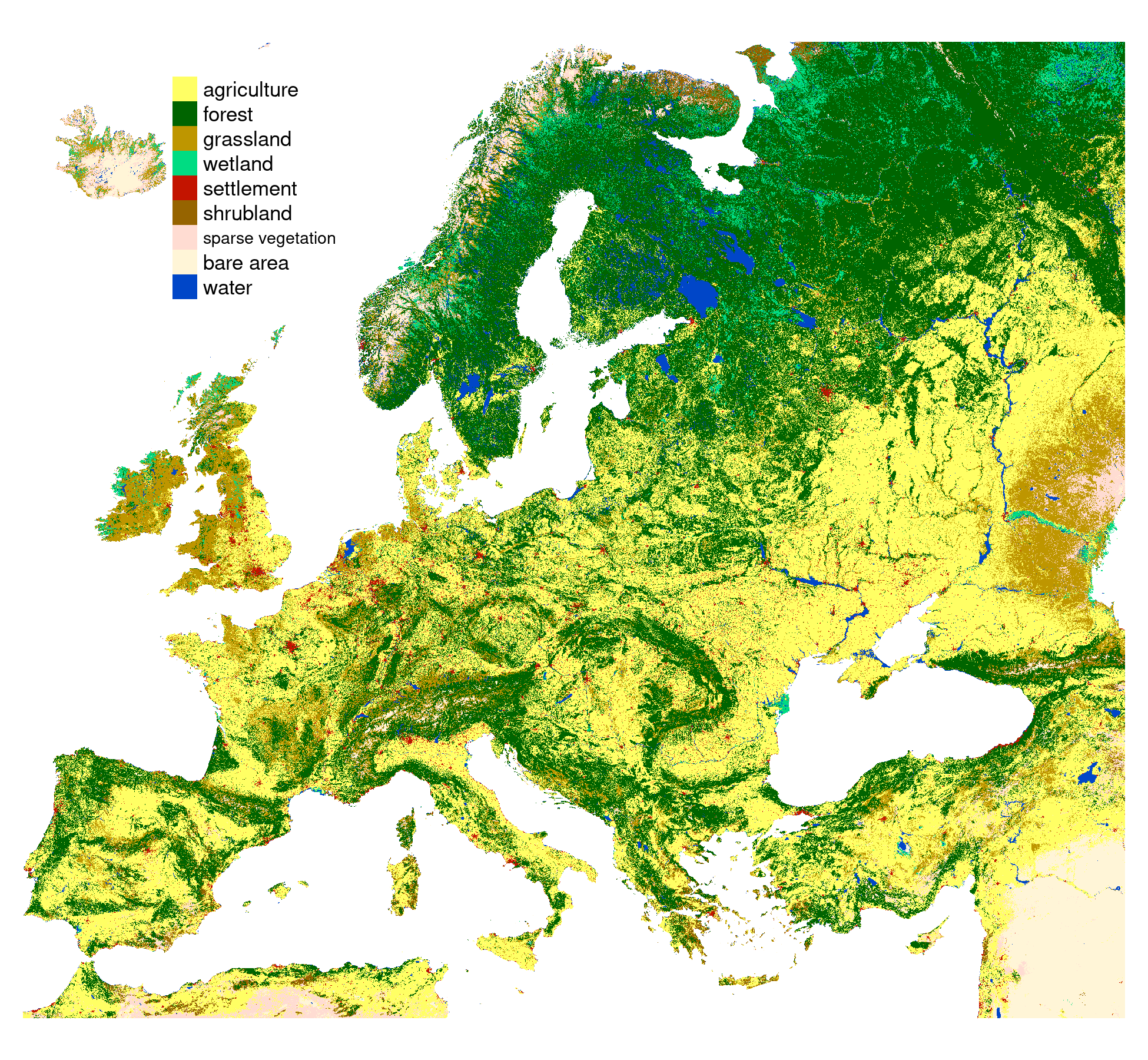
PCA 1 PCA 2 PCA 2 PCA 1 PCA 2 PCA 1 PCA 2 UK EU Entropy Relative mutual information Land cover data Parametrization of two IT metrics Parametrization of two IT metrics