Pattern-based spatial analysis

How to discover and to describe

Chris Reudenbach

Spatial Patterns

In recent years, the ideas of analyzing spatial patterns have been extended through an approach called pattern-based spatial analysis (Long in in. 2010; Cardille in in. 2010; Cardille in in. 2012; Jasiewicz i in. 2013; Jasiewicz i in. 2015).

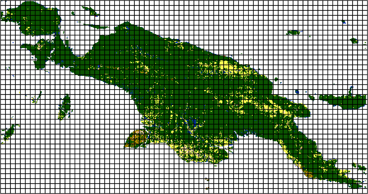
The fundamental idea is to divide a big area into a large number of smaller areas which we may call local landscapes patches.

Note: The patch size is depending on spatial data resolution and scale of the landscape

The idea is to represent each of this arbitrary areas using a statistical description of the spatial pattern - a spatial signature.

This spatial signatures can be compared using a large number of existing distance or dissimilarity measures (Lin 1991; Cha 2007), which enables spatial analyses such as searching, change detection, clustering, or segmentation.

Spatial Signatures

Most landscape metrics are single numbers representing specific features of a local landscape.

Spatial signatures, on the other hand, are multi-element representations of landscape composition and configuration.

The basic signature is the co-occurrence matrix:

Spatial signatures dimension reduction & normalisation

Reduced co-occurrence vector (cove)

Normalized co-occurrence vector(cove)

Co-occurrence vector (cove)

Dissimilarity measures Example 1

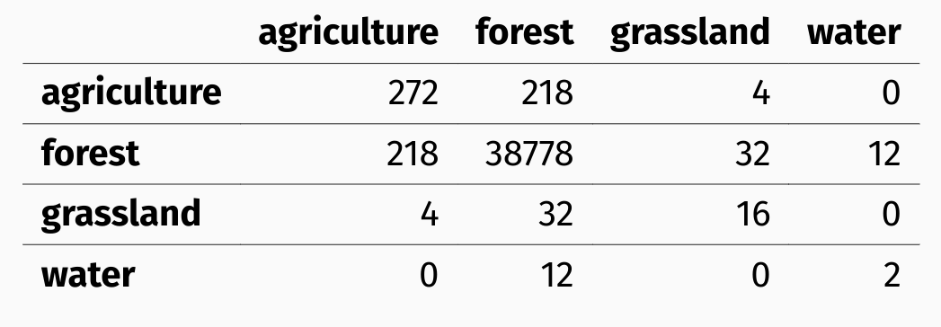
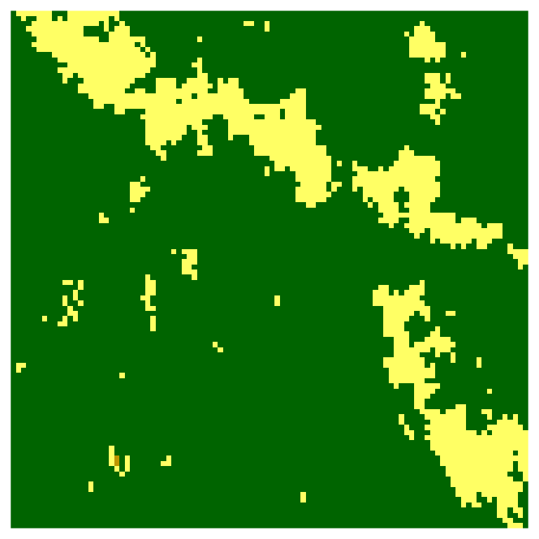
Measuring the distance between two signatures in the form of normalised vectors allows the dissimilarity between spatial structures to be determined. The package [motif] (https://jakubnowosad.com/motif/) is designed to do this work.

Jensen-Shannon distance between the above rasters: 0.0684

Dissimilarity measures Example 2

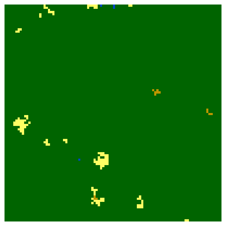
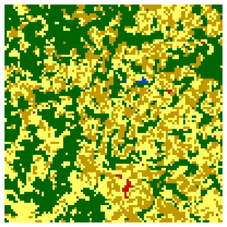
Measuring the distance between two signatures in the form of normalized vectors allows determining dissimilarity between spatial structures.

Jensen-Shannon distance between the above rasters: 0.444

Pattern-based spatial analysis

The distance between spatial signatures provides a powerful possibility to identify (dis)similarities in several contexts.

finding similar spatial structures - one to many comparison

quantitative assessment of changes in spatial structures - one to one comparison

clustering similar spatial structures - many to many comparison

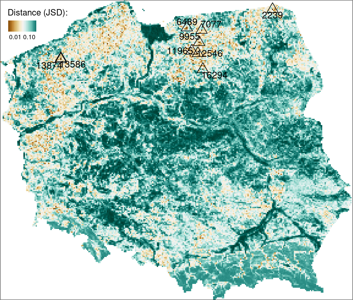
One to many

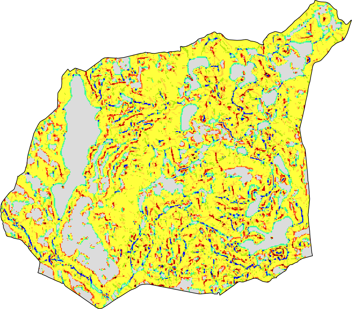
Finding areas with similar topography to the Suwalski Landscape Park

Topography Indices

JSD Index

One to one

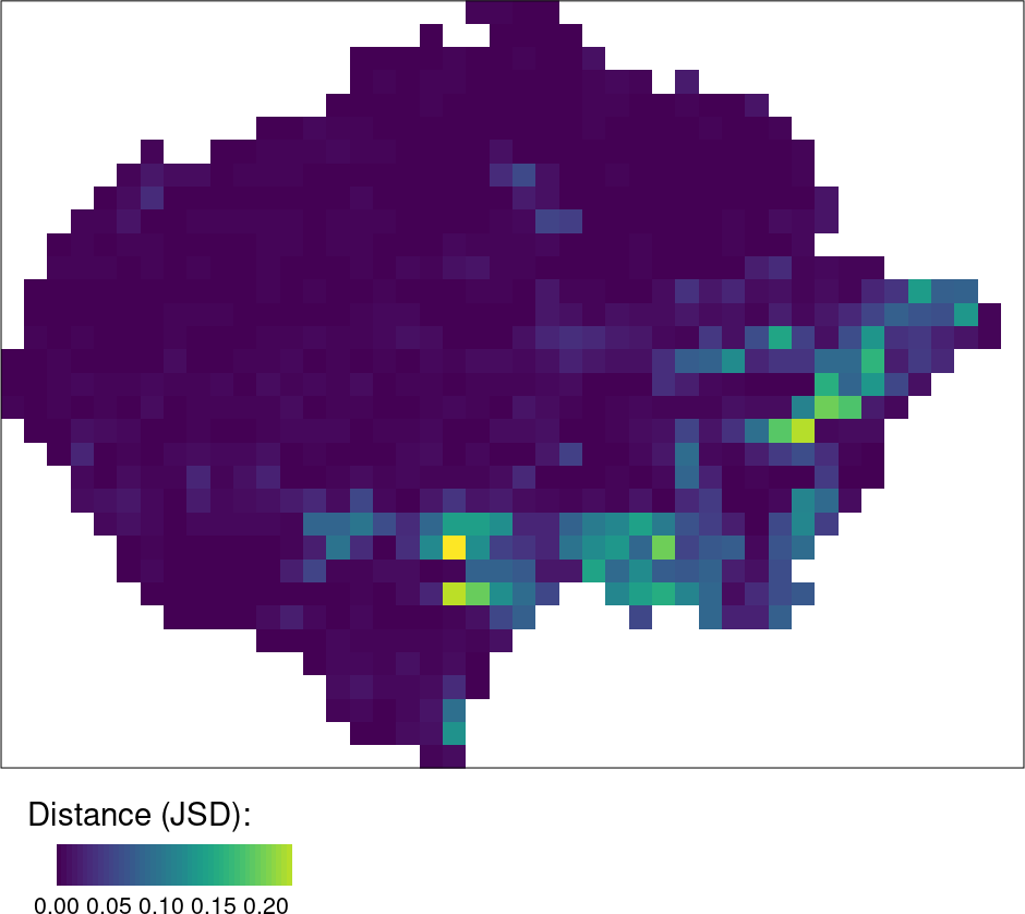
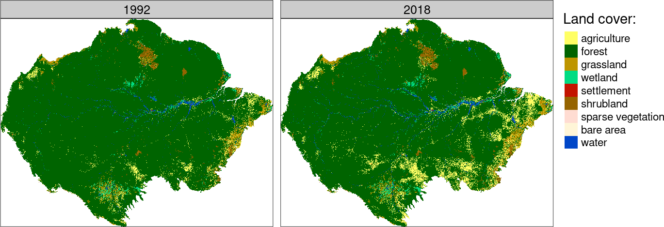
The left maps are showing that many areas in the Amazon have undergone significant land cover changes between 1992 and 2018. The challenge now is to determine which areas have changed the most. The right map shows these areas identified by high JSD values.

Note that changes in both category and spatial configuration are measured.

Landuse Types

JSD Index

Many to many

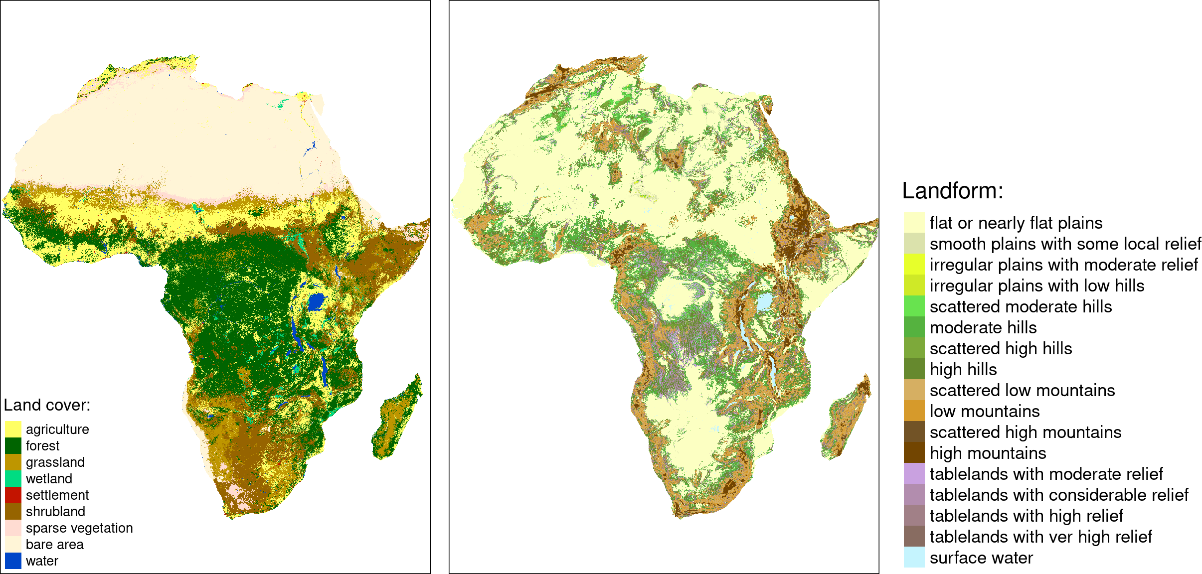
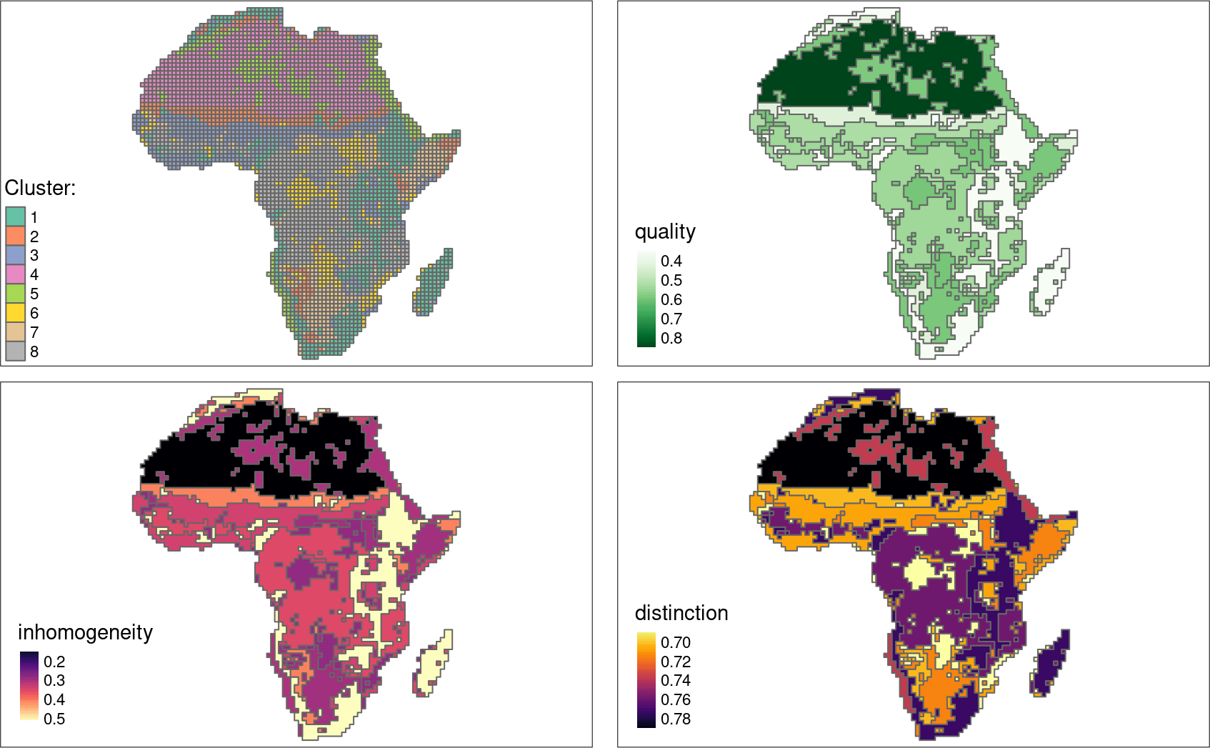
Areas in Africa with similar spatial structures for two themes have been identified - land cover and landforms.

Many to many

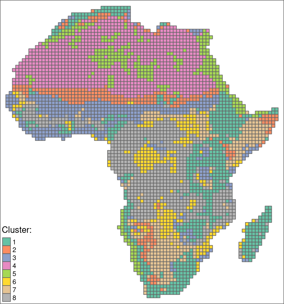
The quality of each cluster can be assessed using metrics:

• Intra-cluster heterogeneity: determines distances between all landscapes within a group
• Inter-cluster isolation: determines distances between a given group and all others

Examples

coma

library(terra)
library(motif)
r9 = rast("../exdata/r9.tif")
r9_sign_coma = lsp_signature(r9, type = "coma")
r9_sign_coma
r9_sign_coma$signature

cove

r9_sign = lsp_signature(r9, type = "cove")
r9_sign
r9_sign$signature

search

library(sf)
landcover = rast(system.file("raster/landcover2015s.tif", package = "motif"))
ecoregions = read_sf(system.file("vector/ecoregionss.gpkg", package = "motif"))
ecoregion1 = ecoregions[1, ]
landcover1 = crop(landcover, ecoregion1, mask = TRUE)
plot(landcover)
plot(landcover1)

search_result = lsp_search(landcover1, landcover, 
                           type = "cove", dist_fun = "jensen-shannon", window = 25,
                           output = "sf")
plot(search_result["dist"])

min/max

search_result$id[which.min(search_result$dist)]
search_results_75 = lsp_extract(landcover, window = 25, id = 75)
plot(search_results_75)

search_result$id[which.max(search_result$dist)]
search_results_215 = lsp_extract(landcover, window = 25, id = 215)
plot(search_results_215)

Exercises

1. Read the study area polygon from the exdata/harz_borders.gpkg file using the read_sf() function from the sf package.
2. Read the land cover raster data for Europe from the file exdata/lc_europe.tif using the function rast() from the package terra. Visualise both datasets.
3. Crop and mask the raster to the polygon boundaries. Visualise the results.
4. Compute a spatial signature for the study area. Can you understand its meaning?
5. Find out which areas of the Europe raster are most similar to the study area (this may take a minute or so). Try different window sizes (e.g. 200 or 500).

Reduced co-occurrence vector (cove) Normalized co-occurrence vector(cove) Co-occurrence vector (cove) Jensen-Shannon distance between the above rasters: 0.0684 Jensen-Shannon distance between the above rasters: 0.444 finding similar spatial structures - one to many comparison quantitative assessment of changes in spatial structures - one to one comparison clustering similar spatial structures - many to many comparison Topography Indices JSD Index Landuse Types JSD Index