Advanced GIS and Remote Sensing - Spatial patterns of non-categorical rasters

Climate data - best practicse

First we need to setup our environment.

install.packages("geodata")
devtools::install_github("Nowosad/spquery")
devtools::install_github("Nowosad/patternogram")
devtools::install_github("Nowosad/supercells")
library(terra); library(sf);library(geodata);library(mapview);library(spquery);library(patternogram)

Using the geodata package (helper package for terra) we can download in a very comfortable often used core data sets. In this case Worldclim and

# German border on top level (nation)
de = geodata::gadm(country = "DEU",level = 0,path = tempdir())
# Worldclim historical climate data for Germany https://www.worldclim.org/data/index.html
wc_tmin_de = worldclim_country("Germany", var="tmin", path=tempdir())
# WCRP Coupled Model Intercomparison Project data https://www.wcrp-climate.org/wgcm-cmip
cmip_tmin_2_5  = geodata::cmip6_world("CNRM-CM6-1", "585", "2061-2080", var="tmin", res=10, path=tempdir())
# cropping and masking
wc_tmin_de = crop(wc_tmin_de,de,mask=T)
cmip_tmin_2_5_de = crop(cmip_tmin_2_5 , de,mask=T)
# set plotting layout
nf <- layout( matrix(c(1,2), ncol=2) )

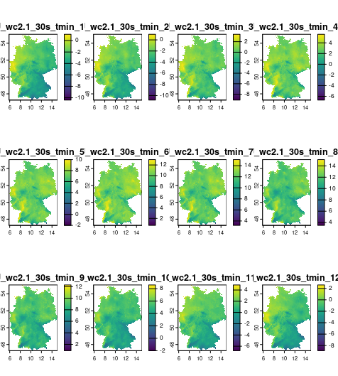
plot(cmip_tmin_2_5_de)
plot(wc_tmin_de)

Note: Please check the websites for the meaning of the data

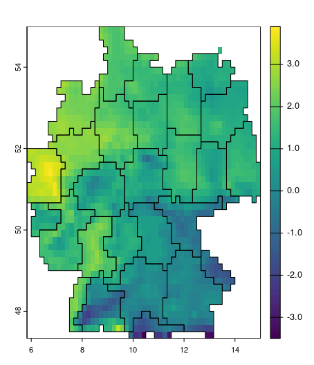
Minimum temperature (°C)

CMIP6 downscaled future climate projection for 2061-2080 [model: CNRM-ESM2-1; ssp: “585”]

WorldClim version 2.1 climate data for 1970-2000

Identifying and comparing similar spatial patterns

Using the package spquery for finding similarities in continous raster data (e.g., raster time-series)

# get Marburg and make it a spatial point
mr = st_sf(st_sfc(st_point(c( 8.770833, 50.810001)),
                  crs = "EPSG:4326"))
vec = as.numeric(extract(wc_tmin_de, mr, ID = FALSE))
vec
# search for similarity in the data set
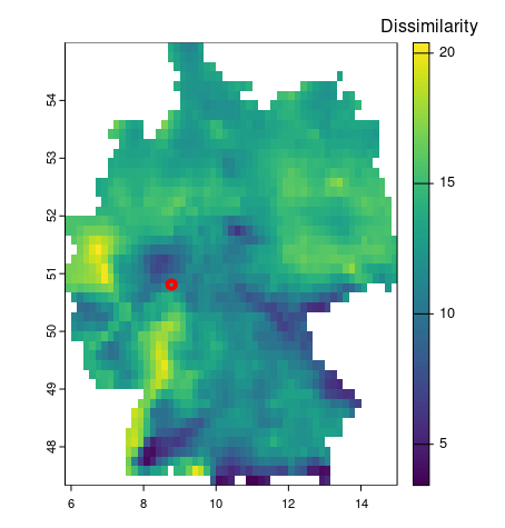
search_tmin = spq_search(vec, cmip_tmin_2_5_de,
                         dist_fun = "euclidean")

# visualize
plot(search_tmin,
     plg = list( loc = "topright",title = "Dissimilarity"))
plot(mr, add=TRUE, col='red', lwd=4)

# some cleaning
crop= crop( wc_tmin_de,cmip_tmin_2_5_de)
res = resample(crop,cmip_tmin_2_5_de)

# call comparison
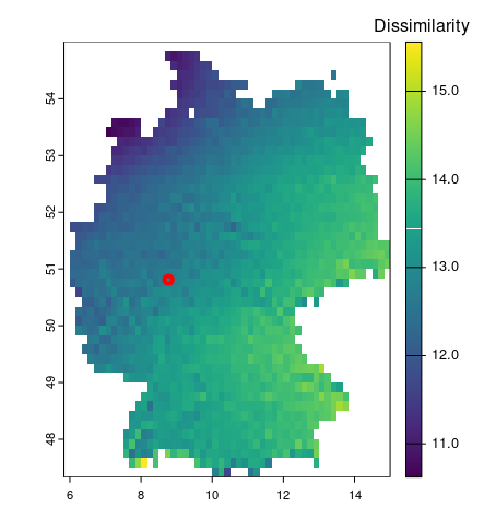
compare_tmin = spq_compare(cmip_tmin_2_5_de, res,
                           dist_fun = "euclidean")

# visualize
plot(compare_tmin,
     plg = list( loc = "topright",title = "Dissimilarity"), 
     col =viridis(256))
plot(mr, add=TRUE, col='red', lwd=4)

patternogram

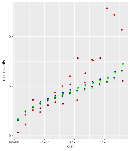
Describing the range of spatial autocorrelation

explore spatial autocorrelations of predictors in machine learning models
detect spatial autocorrelation in various data structures
compare the spatial autocorrelation of variables over time
investigate spatial autocorrelation of categorical spatial patterns

library(patternogram)
library(ggplot2)
pg1_100 = patternogram(wc_tmin_de, sample_size = 10)
pg2_100 = patternogram(cmip_tmin_2_5_de, sample_size = 10)
pg1_500 = patternogram(wc_tmin_de, sample_size = 100)
pg2_500 = patternogram(cmip_tmin_2_5_de, sample_size = 100)
pg1_1000 = patternogram(wc_tmin_de, sample_size = 1000)
pg2_1000 = patternogram(cmip_tmin_2_5_de, sample_size = 1000)
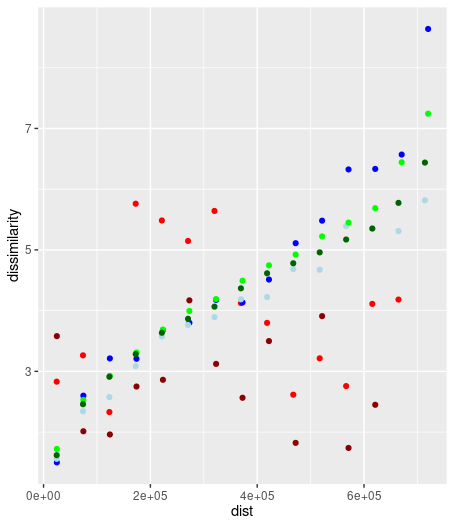
ggplot() + geom_point(data=pg1_100, aes(x=dist, y=dissimilarity), color='red4') +
           geom_point(data=pg2_100, aes(x=dist, y=dissimilarity), color='red') +
           geom_point(data=pg1_500, aes(x=dist, y=dissimilarity), color='blue') +
           geom_point(data=pg2_500, aes(x=dist, y=dissimilarity), color='lightblue') +
           geom_point(data=pg1_1000, aes(x=dist, y=dissimilarity), color='green') +
           geom_point(data=pg2_1000, aes(x=dist, y=dissimilarity), color='darkgreen')

library(patternogram)
library(ggplot2)
pg1_100 = patternogram(wc_tmin_de, width = 100, sample_size = 10)
pg2_100 = patternogram(cmip_tmin_2_5_de, width = 100 ,sample_size = 10)
pg1_500 = patternogram(wc_tmin_de,  width = 100,sample_size = 10)
pg2_500 = patternogram(cmip_tmin_2_5_de,  width = 100,sample_size = 10)
pg1_1000 = patternogram(wc_tmin_de,  width = 100,sample_size = 10)
pg2_1000 = patternogram(cmip_tmin_2_5_de, width = 100,sample_size = 10)
ggplot() + geom_point(data=pg1_100, aes(x=dist, y=dissimilarity), color='red4') +
           geom_point(data=pg2_100, aes(x=dist, y=dissimilarity), color='red') +
           geom_point(data=pg1_500, aes(x=dist, y=dissimilarity), color='blue') +
           geom_point(data=pg2_500, aes(x=dist, y=dissimilarity), color='lightblue') +
           geom_point(data=pg1_1000, aes(x=dist, y=dissimilarity), color='green') +
           geom_point(data=pg2_1000, aes(x=dist, y=dissimilarity), color='darkgreen')

Slic /supercells

supercells: an extension of SLIC (Simple Linear Iterative Clustering; Achanta et al. (2012), doi:10.1109/TPAMI.2012.120) that can be applied to non-imagery geospatial rasters that carry:

pattern information (co-occurrence matrices)
compositional information (histograms)
time-series information (ordered sequences)
other forms of information for which the use of Euclidean distance may not be justified
Segmentation/regionalization: partitioning space into smaller segments while minimizing internal inhomogeneity and maximizing external isolation

SLIC/supercells are a way to improve the output and reduce the cost of segmentation

Code examples

library(terra)
library(supercells)
# Version 1
mintemp_zones = supercells(cmip_tmin_2_5_de, k = 250, compactness = 4)
plot(cmip_tmin_2_5_de[[1]]); plot(mintemp_zones, add = TRUE, col = NA)
# Version 2
mintemp_zones = supercells(cmip_tmin_2_5_de, k = 50, compactness = 4)
plot(cmip_tmin_2_5_de[[1]]); plot(mintemp_zones, add = TRUE, col = NA)
# Version 3
mintemp_zones = supercells(cmip_tmin_2_5_de, k = 250, compactness = 1)
plot(cmip_tmin_2_5_de[[1]]); plot(mintemp_zones, add = TRUE, col = NA)

Code Examples - Helper functions

library(terra)
library(sf)
library(supercells)
library(rgeoda)
library(purrr)
library(tmap)

rawdata="supercells-examples-main/raw-data/"

# create helper functions -------------------------------------------------
get_dtw2d = function(x){
  dist_mat = matrix(nrow = nrow(x), ncol = nrow(x))
  for (i in seq_len(nrow(x))){
    mat1 = matrix(unlist(x[i, ]), ncol = 2)
    for (j in seq_len(nrow(x))){
      mat2 = matrix(unlist(x[j, ]), ncol = 2)
      dist_mat[i, j] = dtwclust::dtw_basic(mat1, mat2, norm = "L2", step.pattern = dtw::symmetric2)
    }
  }
  stats::as.dist(dist_mat)
}
dtw_2d = function(x, y){
  dtw2ddistance = dtwclust::dtw_basic(x = matrix(x, ncol = 2), y = matrix(y, ncol = 2),
                                      norm = "L2", step.pattern = dtw::symmetric2,
                                      error.check = FALSE)
  return(dtw2ddistance)
}

regionalize_dtw_2d = function(k, superpixels, ...){
  weight_df = st_drop_geometry(superpixels[, !colnames(superpixels) %in% c("supercells", "x", "y")])
  weight_dist = get_dtw2d(weight_df)
  rook_w = rook_weights(superpixels)
  skater_results = ?skater(k, rook_w, weight_df, random_seed = 1, cpu_threads = 1, scale_method = "raw",
                          rdist = weight_dist)
  superpixels$cluster = skater_results$Clusters
  regions = aggregate(superpixels, by = list(superpixels$cluster), mean)
  regions = st_cast(regions, "POLYGON")
  regions$k = k
  return(regions)
}

# normalize function
scale_01 = function(r){
 
  # get the min max values
  minmax_r = range(values(r), na.rm=TRUE) 
  
  # rescale 
  return( (r-minmax_r[1]) / (diff(minmax_r)))
}

Code Examples - Regionalisation based on supercells

# create supercells based on the 2D time-series ---------------------------
sp = supercells(c(ta, pr), step = 15, compactness = 0.01, dist_fun = dtw_2d)
plot(sp)

# create 3, 7, 11, and 15 regions based on the 2D time-series -------------
sp_regions = ?map_dfr(c(3, 7, 11, 15), regionalize_dtw_2d, sp)

tm_shape(sp_regions) +
  tm_polygons() +
  tm_facets("k")

Exercises

The goal: to regionalize Germany’s climates

Use Worldclim versus CMIP data
Use the upper helper functions and code for Great Britain

Extended SLIC workflow uses the dynamic time warping (DTW) distance function rather than the Euclidean distance.