Object-based Image Analysis (OBIA)

Human visual perception almost always outperforms computer image processing algorithms. For example, your brain easily recognizes a river, whereas a computer may struggle to distinguish rivers from lakes, roads, or sewage treatment plants.

With UAV image data — which often have high spatial resolution but minimal spectral resolution — a shift in analytical thinking is required. Instead of classifying individual pixels, it is more effective to identify meaningful objects or entities. The core principle of Object-Based Image Analysis (OBIA) is therefore: segment first, then classify.

Segmentation is algorithm-dependent and iteratively searches for similarities in spatial, structural, and spectral dimensions to group neighboring pixels into coherent objects. These segments are subsequently classified using supervised training data.

---

General Workflow

The example below illustrates a typical OBIA classification procedure performed manually in a software environment. The main steps are:

1. Data acquisition (orthophoto, training data)
2. Generation of spatial segments
3. Extraction of suitable descriptive features
4. Model training
5. Classification of the input dataset

In practice, additional steps are often required due to software constraints. Furthermore, the workflow may not be strictly linear, as intermediate results are frequently reused. The following figure shows the step-by-step process in the form of a graphical model. This can be integrated into QGIS as a tool in the Processing Toolbox.

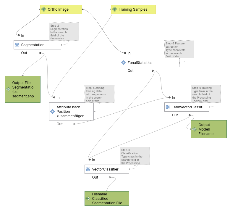
OBIA Classification Workflow for Orthoimages

For reference, you may Download the base dataset. Additionally, you can download the OBIA workflow as a QGIS Model. To add it to your QGIS project, click the first icon “Models” in the Processing Toolbox and choose Add Model to Toolbox. Note that it runs with fixed default values; to modify it, right-click on the model and choose Edit Model.

---

Step-by-Step Tutorial

This step-by-step guide demonstrates an OBIA approach using QGIS and the OTB Toolbox. Many segmentation algorithms and classification methods are available. The Mean-Shift segmentation combined with Support Vector Machine (SVM) classification is robust and commonly used.

Key parameters like Range Radius (feature space) and Spatial Radius (search space), as well as the Minimum Region Size, significantly impact the result and often require empirical fine-tuning.

---

Step 1 – Create Training Sample Points (Manual Digitizing)

If you’re unfamiliar with digitizing in QGIS, follow this tutorial.
Note: For this example, we will digitize points, not polygons.

Create a point vector file and digitize the following classes:

class	CLASS_ID
water	1
meadows	2
meadows-rich	3
bare-soil-dry	4
crop	5
green-trees-shrubs	6
dead-wood	7
other	8

Provide at least 10 widely distributed sampling points per class.
Save the file as sample.gpgk.

---

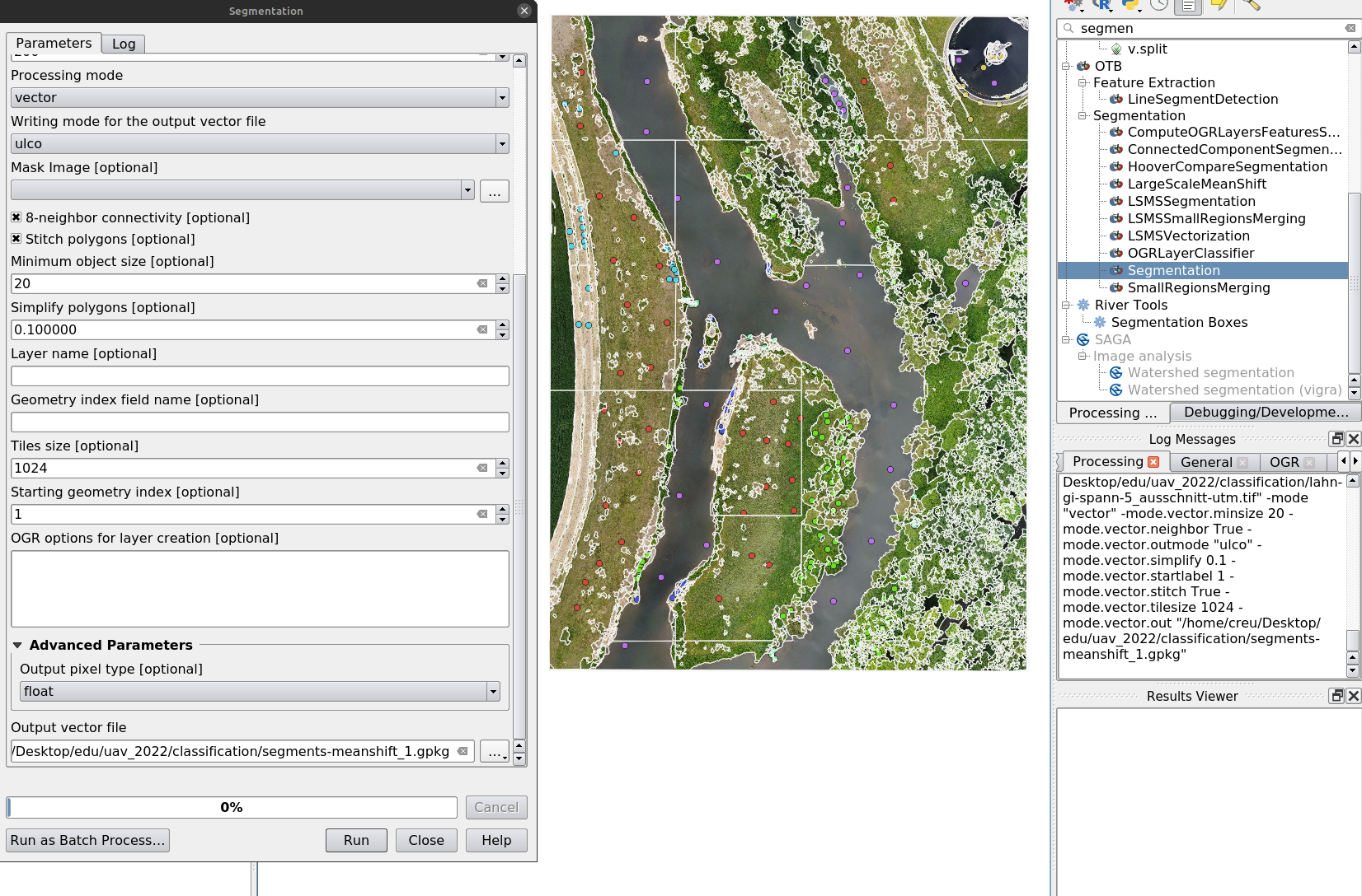
Step 2 – Segmentation

In the QGIS Processing Toolbox, type segmentation and double-click Segmentation.

Configure the parameters:

• Input image: example-5.tif
• Segmentation algorithm: meanshift
• Spatial Radius: 25 (adjust based on the pixel scale of your major classes)
• Range Radius: 25 (based on image type and spectral dynamic)
• Minimum Region size: 25 pixels (small clusters are merged)
• Processing mode: Vector
• Neighborhood: tick 8-neighborhood connectivity
• Minimum object size: 200 pixels
• Output vector file: segments-meanshift.shp

Click Run.

Inspect results:

• Load segments-meanshift.shp into your QGIS project and overlay it on example-5.tif
• Style the segments for visibility:
  Layer Properties → Symbology → Simple Fill:
  Set Fill Style: No Brush and Stroke Color: White
• If the result is unsatisfactory, adjust parameters and repeat.

---

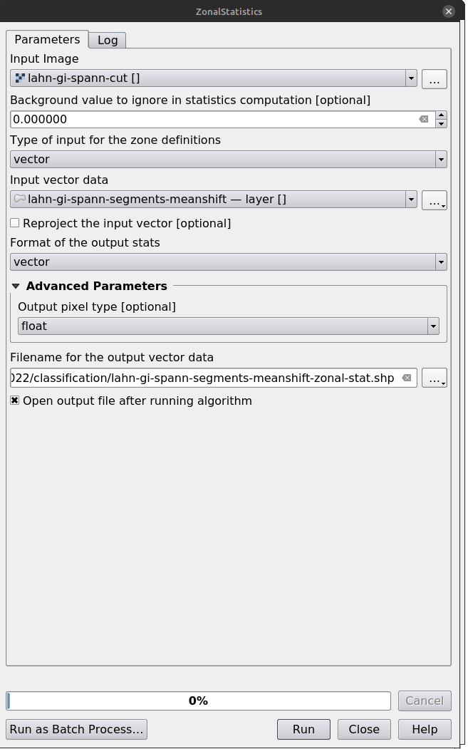
Step 3 – Feature Extraction

In the Processing Toolbox, type zonalstats and open ZonalStatistics (under OTB → Image Manipulation).

• Input image: example-5.tif
• Input vector: segments-meanshift.shp
• Output vector: segments-meanshift-zonal.shp

Click Run.

---

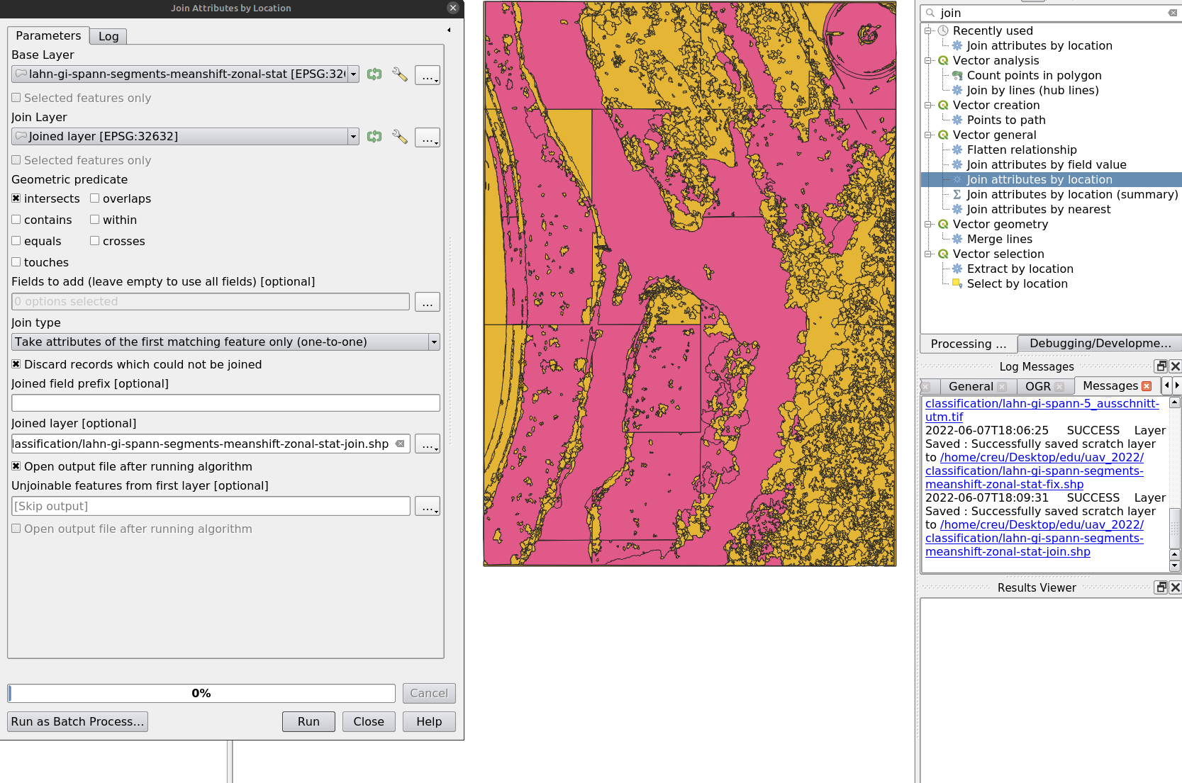
Step 4 – Join Training Data with Segments

In the Processing Toolbox, search for join and open Join Attributes by Location.

Set the parameters:

• Base Layer: segments-meanshift-zonal.shp
• Join Layer: sample.shp
• Join Type: Take Attributes of the first matching feature
• Tick: Discard records which could not be joined
• Output: choose a file name

---

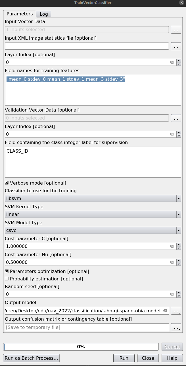
Step 5 – Training

In the Processing Toolbox, type train and open TrainVectorClassifier.

Configure:

• Vector Data List: segments-meanshift-zonal.shp (after join!)
• Output model filename: lahn-gi-spann-obia.model
• Field names for training features:
  "mean_0 stdev_0 mean_1 stdev_1 mean_3 stdev_3 mean_2 stdev_2"
• Class field: CLASS_ID
• Classifier: libsvm
• SVM Kernel Type: linear
• SVM Model Type: csvc
• Parameter Optimization: ON

Click Run.

---

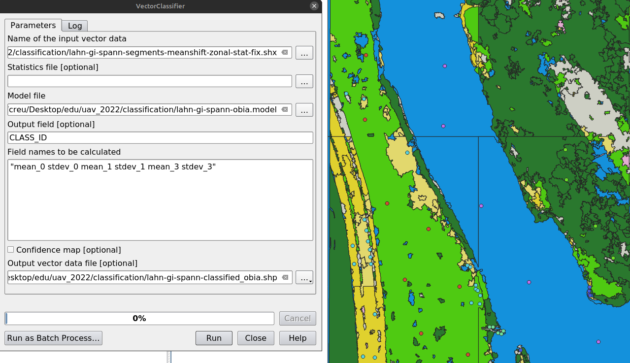
Step 6 – Classification

In the Processing Toolbox, type class and open VectorClassifier.

Configure:

• Input Vector: segments-meanshift-zonal.shp
• Input Model: lahn-gi-spann-obia.model
• Class field: CLASS_ID
• Feature fields:
  "mean_0 stdev_0 mean_1 stdev_1 mean_3 stdev_3 mean_2 stdev_2"
• Output vector: lahn-gi-spann-classified_obia.shp

Click Run.

Finally, load the output vector into QGIS and apply a style:

Layer → Properties → Symbology → Style → Load Style...

---

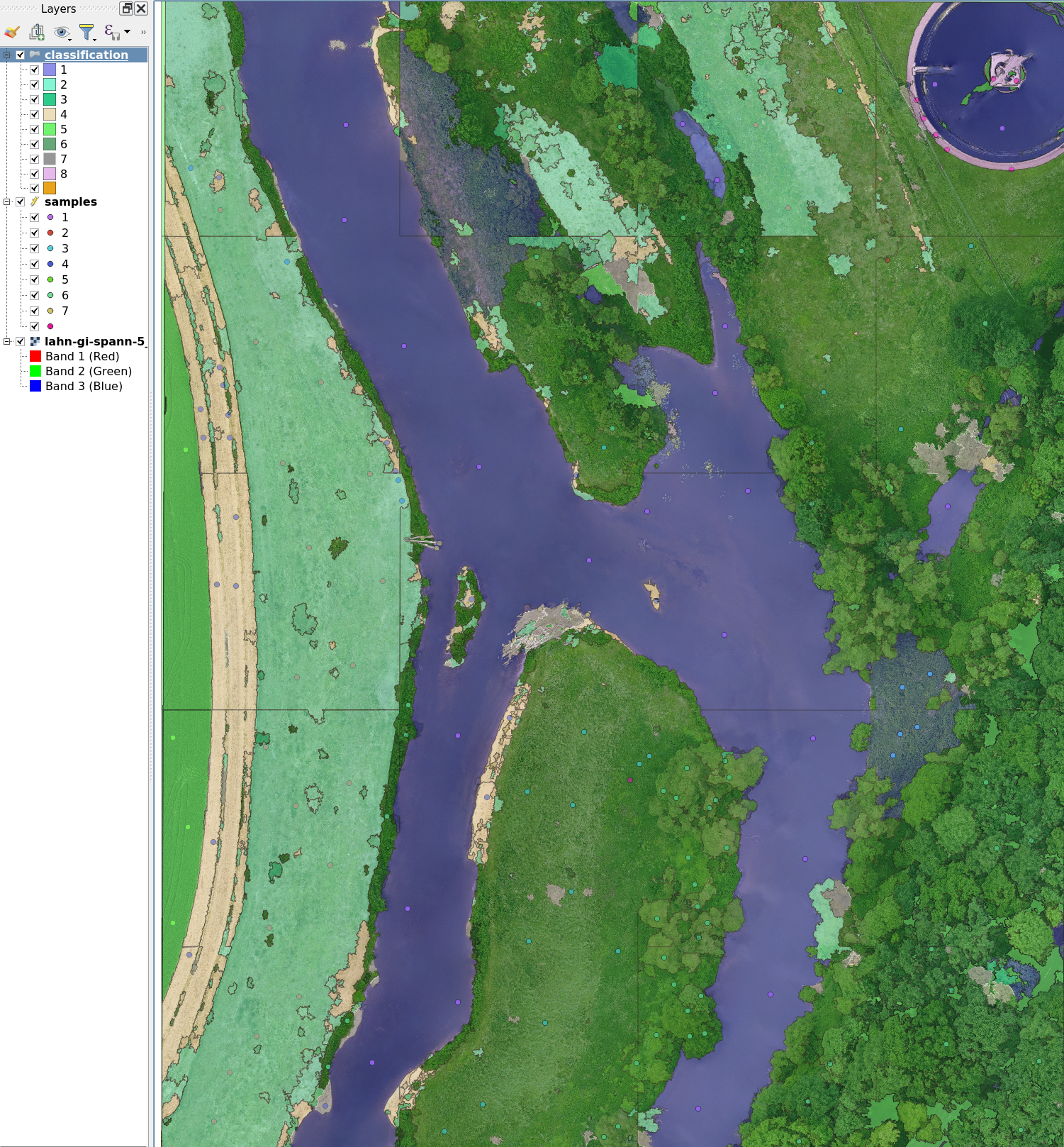
Result

You should now see a mostly well-classified result. However, expect some misclassifications as well.

Questions for further reflection:

• What could be the causes of the misclassifications?
• What are the weaknesses of this approach?
• How could the results be improved?

---