Introduction
Big thanks to Marius Appel, who beside other contributions, gave 2021 at OpenGeoHub Summer School 2021 a great workshop. This blog post builds on that workshop and integrates some additional application aspects.
Sentinel-2 is currently the most important platform for Earth observation in all areas, but especially for climate change, land use and ecological issues at all levels, from the upper micro level to the global level.
There are two operational Sentinel-2 satellites: Sentinel-2A and Sentinel-2B, both in sun-synchronous polar orbits and 180 degrees out of phase. This arrangement allows them to cover the Earth at mid-latitudes with a flyover time of about 5 days.
The Sentinel-2 data are therefore predestined to record spatial and temporal changes on the Earth’s surface (in early summer the forest was green, in late summer it has disappeared). They are ideal for timely studies before and after natural disasters or for biomass balancing, etc.
Cloud-Optimised GeoTIFFs (COGs)
Unfortunately, the official Sentinel-2 archives are anything but really user-friendly. Even with highly convenient toos as sen2r it is sometimes cumbersome to process tTechnically the processed product levels are available to for download preprocessed as L1C and L2A products in JP2K format. Most of the data is stored on the long term storages. the preferred file format is JP2K which is storage efficient but has to be fully downloaded locally by the user and thus have high access costs and huge requirements for local storage space. The Cloud-Optimised GeoTIFFs (COGs) allow only the areas of interest to be loaded and also the processing is significantly faster. However, it requires optimised cloud services and technically a different access logic than in the processing chains used so far.
SpatioTemporal Asset Catalog (STAC)
The SpatioTemporal Asset Catalog (STAC) provides a common language for simplified indexing and searching of geospatial data. A “spatio-temporal asset” is a file that contains information in a specific space and time.
This approach allows all providers of spatio-temporal data (imagery, SAR, point clouds, data cubes, full motion video, etc.) to provide SpatioTemporal Asset Catalogs (STAC) for their data. STAC focuses on an easy to implement standard that organisations can use to make their data available in a durable and reliable way.
Element84 has provided a public API called Earth-search, a central search catalogue for all public AWS datasets using STAC (including the new Sentinel-2 COGs). this contains, beginning 1 November 2017, more than 11.4 million Sentinel-2 scenes worldwide.
Goals
This example shows how complex times series methods from external R packages can be applied in cloud computing environments using [rstac (Brazil Data Cube Team 2021) and gdalcubes (Appel and Pebesma 2019). We will use the bfast R package containing unsupervised change detection methods identifying structural breakpoints in vegetation index time series. Specifically, we will use the bfastmonitor() function to monitor changes on a dedicated timeperiod of a time series of Sentinel-2 imagery.
Other packages used in this tutorial include stars (Pebesma 2019), tmap (Tennekes 2018) and mapview (Appelhans et al. 2022) for creating interactive maps, sf (Pebesma 2018) for processing vector data, and colorspace (Zeileis et al. 2020) for visualizations with accessible colors.
Various approaches to time series and difference analyses with different indices will be applied using the example of the MOF AOI for the time period 1997 - 2021.
Starting the Analysis
Setup the working environment
# adapt your directory this is following the concept of the envimaR structure
tutorialDir = path.expand("~/edu/agis/doc/data/tutorial/")

library(sf)
library(raster)
library(tidyverse)
library(downloader)
library(tmap)
library(tmaptools)
library(mapview)
library(gdalcubes)
library(OpenStreetMap)
library(stars)
library(colorspace)
library(rstac)


ndvi.col = function(n) {
  rev(sequential_hcl(n, "Green-Yellow"))
}

ano.col = diverging_hcl(7, palette = "Red-Green",  register = "rg")
Defining the Area of Interest
One major challenge is the fact that most of the earth surface related remote sensing activities are heavily “disturbed” by the atmosphere, especially by clouds. So to find cloud free satellite imagery is a common and cumbersome task. This task is supported by the rstac package which provides a convenient tool to find and filter adequate Sentinel-2 images out of the COG data storage. However, to address the AOI we need to provide the extend via the bbox argument of the corresponding function stac_search(). So first we need to derive and transform the required bounding box to WGS84 geo-coordinates, easily done with the sf functions st_bbox() and st_transform(). In addition we adapt the projection of the referencing vector objects to all other later projection needs.
Please note to project to three different CRS is for this examples convenience and clarity and somewhat superfluous. Only the corner coordinates of the sections are required and not the complete geometries. However, it creates more clarity for the later process to already have the data needed in different projections.
library(tmap)
library(tmaptools)
utils::download.file(url="https://github.com/gisma/gismaData/raw/master/MOF/MOF_CORE.gpkg",destfile=paste0(tutorialDir,"forest/MOF_CORE.gpkg"))

forest_mask = st_read(paste0(tutorialDir,"forest/MOF_CORE.gpkg"))
## Reading layer `MOF_CORE' from data source
## `/home/creu/edu/agis/doc/data/tutorial/forest/MOF_CORE.gpkg'
## using driver `GPKG'
## Simple feature collection with 50 features and 3 fields
## Geometry type: MULTIPOLYGON
## Dimension: XY
## Bounding box: xmin: 8.662985 ymin: 50.83373 xmax: 8.690624 ymax: 50.84725
## Geodetic CRS: WGS 84sf::st_crs(forest_mask) <- 4326
fm=bb(forest_mask,projection=4326)
forest_4326 =st_transform(forest_mask,crs = 4326)
forest_3035 =st_transform(forest_mask,crs = 3035)
forest_32632 =st_transform(forest_mask,crs = 32632)
# call background map
osm_forest <- tmaptools::read_osm(fm,type = "bing")
# mapping the extents and boundaries of the choosen geometries
tmap_mode("view")## tmap mode set to interactive viewingtmap_options(check.and.fix = TRUE) +
tm_basemap(server = c("Esri.WorldGrayCanvas", "OpenStreetMap", "Esri.WorldTopoMap","Esri.WorldImagery")) +
tm_shape(forest_mask) +
tm_polygons(alpha = 0.4, col="mainTreeSp")Our study area is pretty small, covering roughly 2.5 by 2.5 km forest area northwest of Marburg. The core part of the AOI is the Marburg Open Forest (MOF) a field research facility of the Philipps University Marburg.
Querying images with rstac
Using the rstac package, we first request all available images from 2017 to 2020 that intersect with our region of interest. Here, since the polygon has WGS84 as CRS, we do not need to transform the bounding box before using the stac_search() function.
# search the data stack for the given period and area
library(rstac)

s = stac("https://earth-search.aws.element84.com/v0")
items <- s |>
  stac_search(collections = "sentinel-s2-l2a-cogs",
              bbox = c(st_bbox(forest_4326)["xmin"],
                       st_bbox(forest_4326)["ymin"],
                       st_bbox(forest_4326)["xmax"],
                       st_bbox(forest_4326)["ymax"]),
              datetime = "2017-01-01/2021-12-31",
              limit = 1000) |>
  post_request()
items
## ###STACItemCollection
## - matched feature(s): 294
## - features (294 item(s) / 0 not fetched):
## - S2B_32UMB_20211230_0_L2A
## - S2A_32UMB_20211225_0_L2A
## - S2B_32UMB_20211220_0_L2A
## - S2A_32UMB_20211215_0_L2A
## - S2B_32UMB_20211210_0_L2A
## - S2A_32UMB_20211205_0_L2A
## - S2B_32UMB_20211130_0_L2A
## - S2A_32UMB_20211125_0_L2A
## - S2B_32UMB_20211120_0_L2A
## - S2A_32UMB_20211115_0_L2A
## - ... with 284 more feature(s).
## - assets:
## thumbnail, overview, info, metadata, visual, B01, B02, B03, B04, B05, B06, B07, B08, B8A, B09, B11, B12, AOT, WVP, SCL
## - other field(s):
## type, stac_version, stac_extensions, context, numberMatched, numberReturned, features, links# print date and time of first and last images
range(sapply(items$features, function(x) {x$properties$datetime}))## [1] "2017-01-10T10:34:07Z" "2021-12-30T10:36:44Z"This gives us 294 matching images recorded between Januar 2017 and December 2021.
Creating a monthly Sentinel-2 data cube
To build a regular monthly data cube, we again need to create a gdalcube image collection from the STAC query result. Notice that to include the SCL band containing per-pixel quality flags (classification as clouds, cloud-shadows, and others), we need to explicitly list the names of the assets. We furthermore ignore images with 50 % or more cloud coverage.
library(gdalcubes)
assets = c("B01","B02","B03","B04","B05","B06", "B07","B08","B8A","B09","B11","SCL")
s2_collection = stac_image_collection(items$features, asset_names = assets, property_filter = function(x) {x[["eo:cloud_cover"]] < 50})
## Warning in stac_image_collection(items$features, asset_names = assets,
## property_filter = function(x) {: STAC asset with name 'SCL' does not include
## eo:bands metadata and will be considered as a single band sources2_collection## Image collection object, referencing 91 images with 12 bands
## Images:
## name left top bottom right
## 1 S2B_32UMB_20211220_0_L2A 7.560563 51.45109 50.45528 9.140444
## 2 S2A_32UMB_20211125_0_L2A 7.560563 51.45109 50.45528 9.140444
## 3 S2A_32UMB_20211016_0_L2A 7.560563 51.45109 50.45528 9.140444
## 4 S2B_32UMB_20211001_0_L2A 7.560563 51.45109 50.45528 9.140444
## 5 S2A_32UMB_20210926_0_L2A 7.560563 51.45109 50.45528 9.140444
## 6 S2B_32UMB_20210911_0_L2A 7.560563 51.45109 50.45528 9.140444
## datetime srs
## 1 2021-12-20T10:36:43 EPSG:32632
## 2 2021-11-25T10:36:48 EPSG:32632
## 3 2021-10-16T10:36:54 EPSG:32632
## 4 2021-10-01T10:36:48 EPSG:32632
## 5 2021-09-26T10:36:52 EPSG:32632
## 6 2021-09-11T10:36:44 EPSG:32632
## [ omitted 85 images ]
##
## Bands:
## name offset scale unit nodata image_count
## 1 B01 0 1 91
## 2 B02 0 1 91
## 3 B03 0 1 91
## 4 B04 0 1 91
## 5 B05 0 1 91
## 6 B06 0 1 91
## 7 B07 0 1 91
## 8 B08 0 1 91
## 9 B09 0 1 91
## 10 B11 0 1 91
## 11 B8A 0 1 91
## 12 SCL 0 1 91The result contains 91 images which means roughly 1.5 images per month, from which we can now create a data cube. For doinfg so we will use the transformed (UTM) bounding box of our polygon as spatial extent, 10 meter spatial resolution, bilinear spatial resampling (for the coarsere Sentinel channels) and also defined derive monthly median values for all pixel values from the available images within a month. Notice that we add a border seam to each side of the cube.
The gdalcube image collection can be considered as a proxy structure object which will be applied on the COGs.
b = 50
v = cube_view(srs = "EPSG:32632",
              dx = 10,
              dy = 10,
              dt = "P1M",
              aggregation = "median",
              extent = list(t0 = "2017-01",
                            t1 = "2021-12",
                            left = st_bbox(forest_32632)["xmin"] - b,
                            right = st_bbox(forest_32632)["xmax"] + b,
                            bottom = st_bbox(forest_32632)["ymin"] - b,
                            top = st_bbox(forest_32632)["ymax"] + b),
              resampling = "bilinear")
v
## A data cube view object
##
## Dimensions:
## low high count pixel_size
## t 2017-01 2021-12 60 P1M
## y 5631333.77349894 5632943.77349894 161 10
## x 476218.413068451 478268.413068451 205 10
##
## SRS: "EPSG:32632"
## Temporal aggregation method: "median"
## Spatial resampling method: "bilinear"Next, we create a data cube, subset the red and near infrared bands and crop by our polygon, which simply sets pixel values outside of the polygon to NA. Afterwards we save the data cube as a single netCDF file. Notice that this is not neccessary but storing intermediate results makes debugging sometimes easier, especially if the methods applied afterwards are computationally intensive.
Only calling a final action will start the processing on the COG-Server. In this case ‘write_ncdf’.
# we "download" the data and write it t a netcdf file
if (!file.exists((file.path(tutorialDir,"MOF_10.nc"))))
{
  s2.mask = image_mask("SCL", values = c(3,8,9))
  gdalcubes_options(parallel = 24, ncdf_compression_level = 5)
  raster_cube(s2_collection, v, mask = s2.mask) |>
    write_ncdf(file.path(tutorialDir,"MOF_10.nc"),overwrite=TRUE)
}
We will show in the following examples a straightforward plotting in a generic pipe. However a more common visualization is pretty straighforward. A typical pipe could be: Save a resulting netCDF file -> Convert it to a stars object -> Visualize the results with tmap, mapview, ggplot2 or whatever preferred package to create (interactive) map(s).
Reductions
Possible reducers include "min", "mean", "median", "max", "count" (count non-missing values), "sum", "var" (variance), and "sd" (standard deviation). Reducer expressions are always given as a string starting with the reducer name followed by the band name in parentheses. Notice that it is possible to mix reducers and bands.
Counting
To get an idea of the data, we can compute simple summary statistics applying a reducer function over dimensions. For example using the count reducer we learn about the temporal coverage for each aggregated pixel and hence an initial understanding of the data set temporal quality.
ncdf_cube(file.path(tutorialDir,"MOF_10.nc")) |>
  reduce_time("count(B04)") |>
  plot(key.pos = 1, zlim=c(25,45), col = viridis::viridis, nbreaks = 10)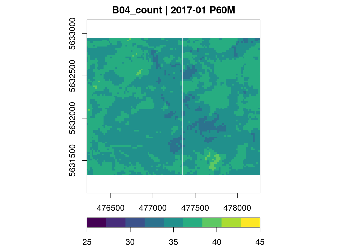
We can see that most time series contain valid observations about 40 months, which should be sufficient for our example. Similarly, it is also possible to reduce over space, leading to summary time series.
Below you will find various examples dealing with the common NDVI and the kNDVI Indices.
kNDVI
Below, we derive mean monthly kNdvi values over all pixel time series.
ncdf_cube(file.path(tutorialDir,"MOF_10.nc")) |>
    apply_pixel("tanh(((B08-B04)/(B08+B04))^2)", "kNDVI") |>
  reduce_time("mean(kNDVI)") |>
  plot(key.pos = 1,  col = ndvi.col, nbreaks = 12)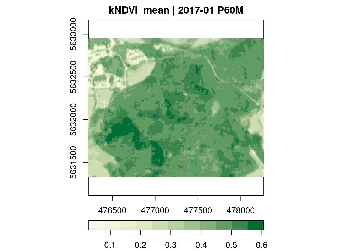
NDVI
Below, we derive mean monthly Ndvi values over all pixel time series.
ncdf_cube(file.path(tutorialDir,"MOF_10.nc")) |>
  apply_pixel("(B08-B04)/(B08+B04)", "NDVI") |>
  reduce_time("mean(NDVI)") |>
  plot(key.pos = 1, zlim=c(-0.2,1), col = ndvi.col, nbreaks = 12)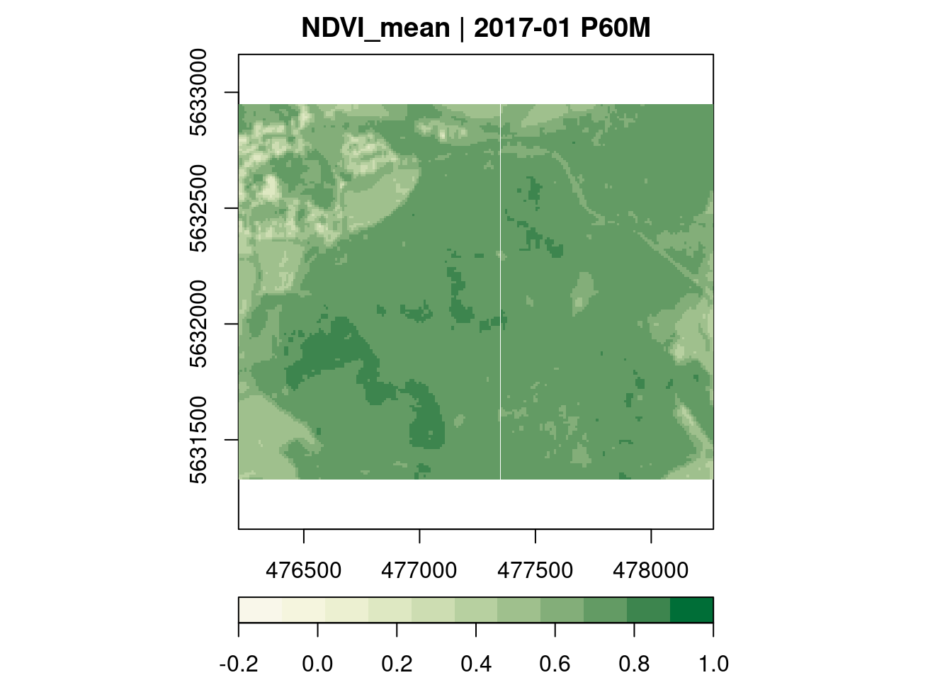
Zonal Statistics
zstats = ncdf_cube(file.path(tutorialDir,"MOF_10.nc")) |>
  apply_pixel("(B08-B04)/(B08+B04)", "NDVI") |>
  extract_geom(forest_32632,FUN = median)

forest_32632$FID = rownames(forest_32632)
x = merge(forest_32632, zstats, by = "FID")
mapview(x[x$time == "2018-07", "NDVI"],col.regions = ndvi.col)
Timeseries
ncdf_cube(file.path(tutorialDir,"MOF_10.nc")) |>
  apply_pixel("tanh(((B08-B04)/(B08+B04))^2)", "kNDVI") |>
  reduce_space("min(kNDVI)", "max(kNDVI)", "mean(kNDVI)") |>
  plot(join.timeseries = TRUE)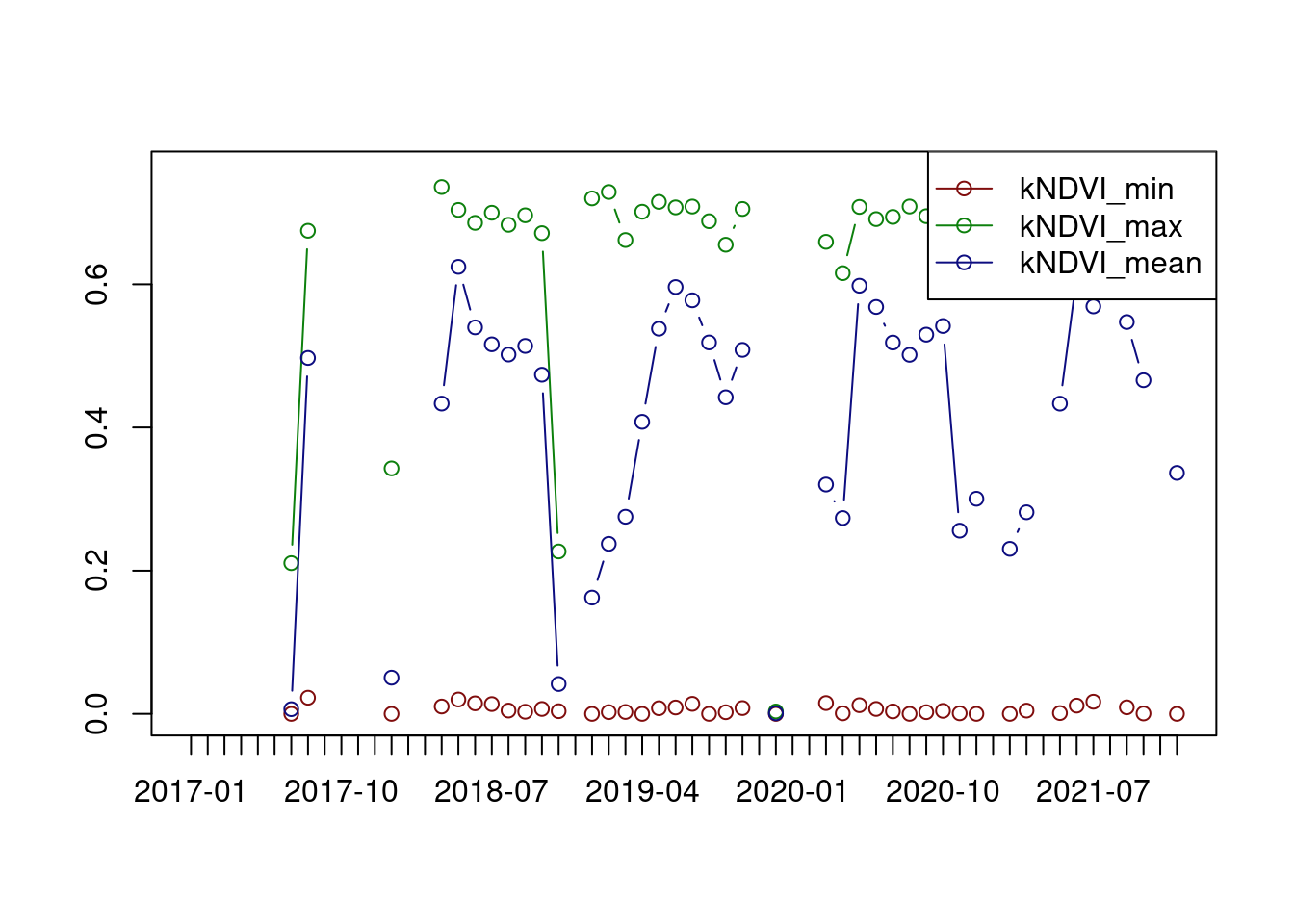
Calculate the annual NDVI difference - using functions
The following function will iterate through 3 years of NDVI data and calculating NDVI difference maps for each pair of years.
gdalcubes_options(parallel =  12)

# ndvi operand
ndvi_type = "median(kNDVI)"

# time slots as tibble
ts = tibble(t0 = c("2018-04-01","2019-04-01","2020-04-01","2021-04-01"),
            t1= c("2018-09-01","2019-09-01","2020-09-01","2021-09-01"))

# names of the time slots
names_ndvi = paste(ts$t0,ts$t1,sep = " to ")

basic_kndvi <- function(fncube=NULL, t0=NULL, t1=NULL) {
  ncdf_cube(fncube) |>
    select_bands(c("B04", "B08")) |>
    select_time(c(t0,t1)) |>
  apply_pixel("tanh(((B08-B04)/(B08+B04))^2)", "kNDVI") |>
    reduce_time(ndvi_type)
}

# (stac-search -> stac and cloud filter image collection -> create cube -> call user function)
ndvi = list()
for (i in 1:nrow(ts)){
  # call user function
  basic_kndvi(fncube = file.path(tutorialDir,"MOF_10.nc"), t0 = ts$t0[i], t1 = ts$t1[i]) %>%
    st_as_stars() -> ndvi[[i]]

}

# now we may create a mask according to the NDVI extent and resolution
stars::write_stars(ndvi[[1]] * 0, paste0(tutorialDir,"forest/only_forestmask.tif"))
gi=link2GI::linkGDAL(searchLocation = "/usr/bin/")
cmd=gi$bin[[1]]$gdal_bin[14]
system(paste(cmd ,'-burn 1.0 -tr 10.0 10.0 -a_nodata 0.0 -te ', st_bbox(ndvi[[1]])$xmin,' ',st_bbox(ndvi[[1]])$ymin,' ',st_bbox(ndvi[[1]])$xmax,' ',st_bbox(ndvi[[1]])$ymax,' -ot Float32 -of GTiff', paste0(tutorialDir,"forest/MOF_mask_pr.shp "),paste0(tutorialDir,"forest/only_forestmask.tif")))
mask <- raster(paste0(tutorialDir,"forest/only_forestmask.tif"))
plot(mask) 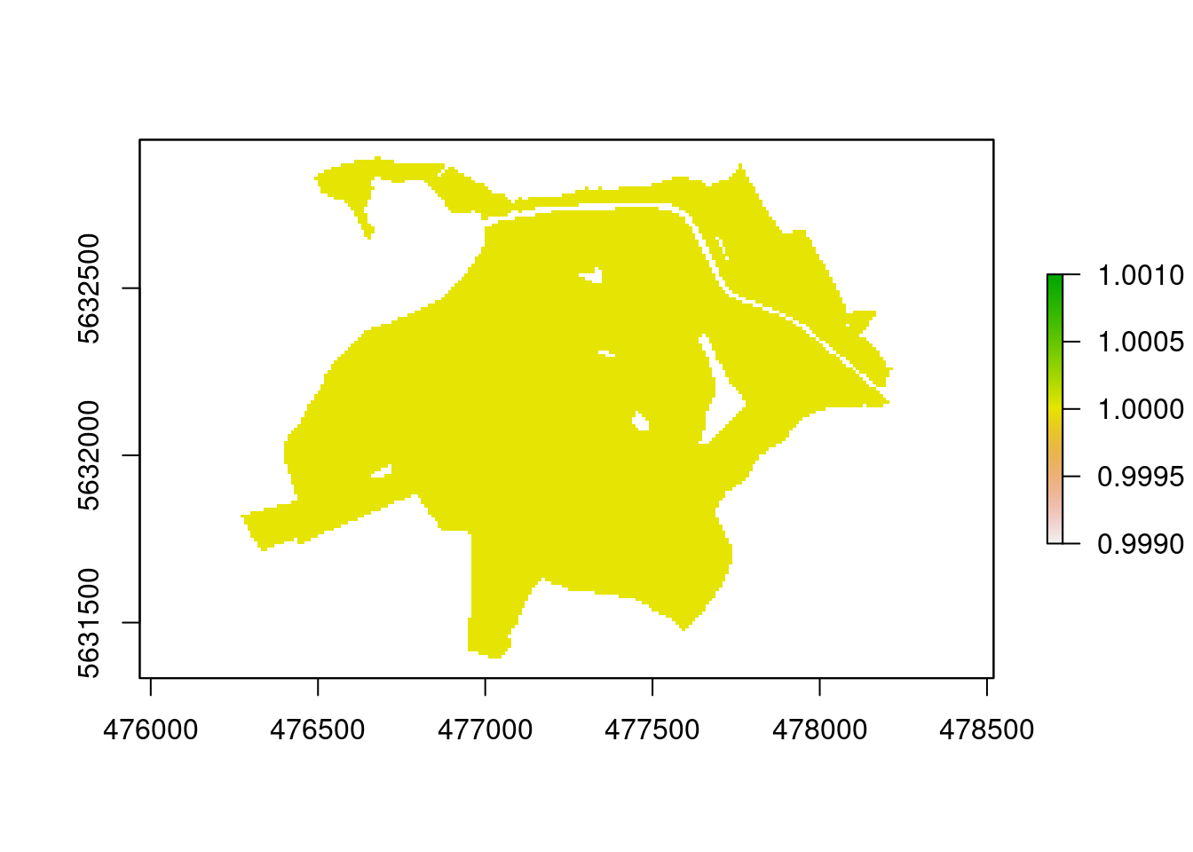
mask[mask == 0] = NA

# mapping the results
tmap_mode("plot")
## tmap mode set to plottingtm_ndvi = lapply(seq(2:length(names_ndvi) -1),function(i){
m = tm_shape(osm_forest) + tm_rgb() +
tm_shape((ndvi[[i]] - ndvi[[i+1]]) * st_as_stars(mask )) +
tm_raster(title = ndvi_type,pal =diverging_hcl(11, "rg")) +
tm_layout(panel.labels = paste("Difference ",names_ndvi[[i]],"/",names_ndvi[[i+1]]),
legend.show = TRUE,
panel.label.color = "darkblue",
panel.label.size =0.5,
panel.label.height=1.2,
legend.text.size = 0.3,
legend.outside = TRUE) +
tm_grid()
})
# tmap_arrange(tm_ndvi,nrow = 1,asp = NA,widths = c(0.33,0.33,0.33),outer.margins = 0.001)Resulting maps
## stars object downsampled to 1136 by 879 cells. See tm_shape manual (argument raster.downsample)## Variable(s) "NA" contains positive and negative values, so midpoint is set to 0. Set midpoint = NA to show the full spectrum of the color palette.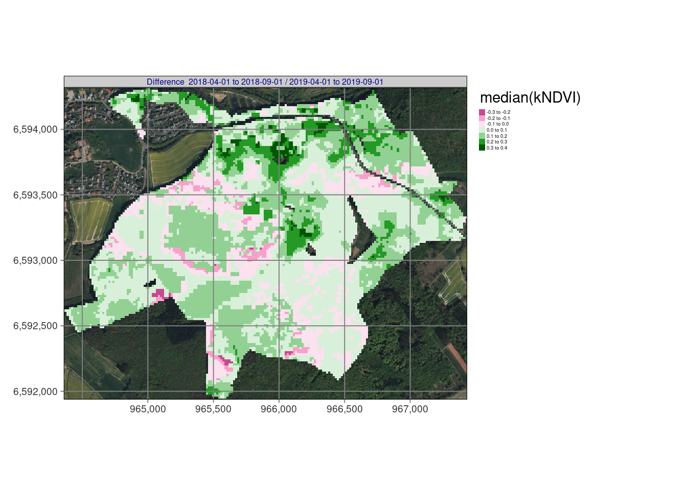
## stars object downsampled to 1136 by 879 cells. See tm_shape manual (argument raster.downsample)
## Variable(s) "NA" contains positive and negative values, so midpoint is set to 0. Set midpoint = NA to show the full spectrum of the color palette.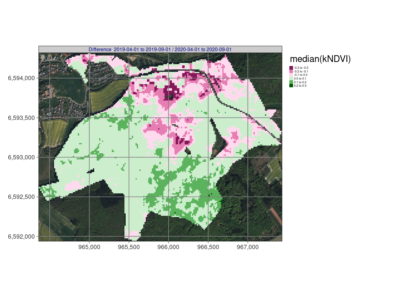
## stars object downsampled to 1136 by 879 cells. See tm_shape manual (argument raster.downsample)
## Variable(s) "NA" contains positive and negative values, so midpoint is set to 0. Set midpoint = NA to show the full spectrum of the color palette.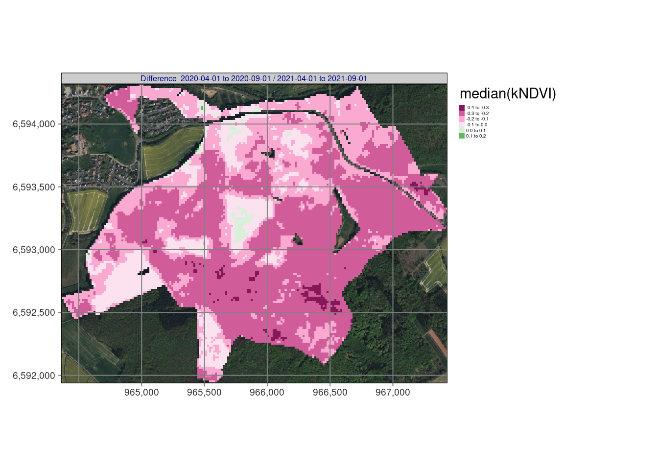
Use case: Spatial identification of magnitudes and time periods of kNDVI changes
To apply a more complex time series method such as bfastmonitor(), the data cube operations below allow to provide custom user-defined R functions instead of string expressions, which translate to built-in reducers. It is very important that these functions receive arrays as input and must return arrays as output, too. Depending on the operation, the dimensionality of the arrays is different:
| Operator | Input | Output |
|---|---|---|
apply_pixel |
Vector of band values for one pixel | Vector of band values of one pixel |
reduce_time |
Multi-band time series as a matrix | Vector of band values |
reduce_space |
Three-dimensional array with dimensions bands, x, and y | Vector of band values |
apply_time |
Multi-band time series as a matrix | Multi-band time series as a matrix |
There is almost no limit of what R function we use, but we must take care of a few things:
1. The reducer function is executed in a new R process without access to the current workspace. It is not possible to access variables defined outside of the function and packages must be loaded within the function.
2. The reducer function must always return a vector with the same length (for all time series).
3. It is a good idea to think about NA values, i.e. you should check whether the complete time series is NA, and that missing values do not produce errors.
Another possibility to apply R functions to data cubes is of course to convert data cubes to stars objects and use the stars package for further analysis.
Applying bfastmonitor as a user-defined reducer function
In our example, bfastmonitor returns change date and change magnitude values per time series so we can use reduce_time(). The script below (1) calculates the kNDVI, (2) applies bfastmonitor(), and properly handles errors e.g. due to missing data with tryCatch(), and (3) finally writes out the resulting change dates and magnitudes of change for all pixels of the time series as a netCDF file. The results shows the changes starting at 1/2019 until 12/2021 and identify pretty well the dynamical impacts of drought and bark beetle in the Marburg University Forest (MOF).
library(sf)
library(tmap)
library(tmaptools)
library(gdalcubes)
library(stars)
library(colorspace)
ndvi.col = function(n) {
  rev(sequential_hcl(n, "Green-Yellow"))
}
tutorialDir = path.expand("~/edu/agis/doc/data/tutorial/")

figtrim <- function(path) {
  img <- magick::image_trim(magick::image_read(path))
  magick::image_write(img, path)
  path
}
gdalcubes_options(parallel = 12)
## start analysis
system.time(
  ncdf_cube(file.path(tutorialDir,"MOF_10.nc")) |>
    reduce_time(names = c("change_date", "change_magnitude","kndvi"), FUN = function(x) {
      kndvi = tanh(((x['B08',]-x['B04',])/(x['B08',]+x['B04',]))^2)
      if (all(is.na(kndvi))) {
        return(c(NA,NA))
      }
      kndvi_ts = ts(kndvi, start = c(2017, 1), frequency = 12)
      library(bfast)
      tryCatch({
        result = bfastmonitor(kndvi_ts, start = c(2020,1),
                              history = "all", level = 0.01)
        return(c(result$breakpoint, result$magnitude))
      }, error = function(x) {
        return(c(NA,NA))
      })
    }) |>
    write_ncdf(paste0(tutorialDir,"bf_results.nc"),overwrite = TRUE))
## User System verstrichen
## 65.435 1.649 16.541Now we can use the netCDF file and map the results with any preferred visualisation tool. In this case tmap.
library(tmap)

mask <- raster(paste0(tutorialDir,"forest/only_forestmask.tif"))
# plotting it from the local ncdf
tmap_mode("view")
gdalcubes::ncdf_cube(paste0(tutorialDir,"bf_results.nc")) |>
  stars::st_as_stars() -> x
tm_shape(osm_forest) + tm_rgb() +
  tm_shape(x[1] * st_as_stars(mask )) +
  tm_raster(n = 6)  +
  tm_layout(
    legend.show = TRUE,
    panel.label.height=0.6,
    panel.label.size=0.6,
    legend.text.size = 0.4,
    legend.outside = TRUE) +
  tm_grid()

tm_shape(osm_forest) + tm_rgb() +
  tm_shape(x[2]* st_as_stars(mask ))  + tm_raster() +
  tm_layout(legend.title.size = 1,
            panel.label.height=0.6,
            panel.label.size=0.6,
            legend.text.size = 0.4,
            legend.outside = TRUE) +
  tm_grid()
Running bfastmonitor() is computationally expensive. However, since in common (not in our case) the data should be located in the cloud, it would be obvious to launch one of the (payed) more powerful machine instance types with many processors. Parallelization within one instance can be controlled entirely by gdalcubes using gdalcubes_options() which is extremely simple.
From a scientific point of view we need to tune some aspects. The kNDVI Index together with the bfastmonitor approach is somewhat sophisticated and need a validation strategy. Also the correlation to the different tree species could be promising. So there is certainly a need for more analysis to understand the processes and to identify false results.
Summary
This examples have shown, how simple and more more complex methods can be applied on data cubes. Especially the chosen approach to just “download” the data from a COG server and perform the processing on the local machine is kind of promising due to the fact that the code can be run almost identically on a cloud instance. The use of more common or well known functionalities and packages helps a lot migrating to gdalcubes concept.
It is even more powerful to use this workflow for extremely comfortable multisensor multiscale approaches.
References
Questions and mistakes but also suggestions and solutions are welcome.
Due to an occasionally faulty page redirection, a 404 error may occur. please use the alternative