Basic Energy Flux Analysis from Energy Balance Station

Author

Chris Reudenbach

Published

July 16, 2025

Introduction

This tutorial calculates surface energy balance components using micrometeorological observations from an energy balance station. We implement a simplified diagnostic approach based on physical theory and field measurements.

Surface Energy Balance: Theory and Interpretation

Understanding the surface energy balance is essential for quantifying the partitioning of energy into heating, evaporation, and ground storage. This notebook follows a physically grounded approach to derive the key energy fluxes from field observations.

Basic Surface Energy Balance Equation

The fundamental balance at the land surface is:

\[ R_n = H + LE + G + S \]

Where:

$R_n$: Net radiation $W/m²$ — total energy input from shortwave and longwave radiation
$H$: Sensible heat flux $W/m²$ — convective transfer of heat to the air
$LE$: Latent heat flux $W/m²$ — energy used for evapotranspiration
$G$: Ground heat flux $W/m²$ — conduction of heat into the soil
$S$: Storage term (e.g. canopy heat, biomass, or air column storage; neglected here)

Assumption: For half-hourly or hourly timesteps and shallow sensors, we assume $S \approx 0$$.
Therefore, we estimate:

\[LE = R_n - G - H\] ### Data Used in This Analysis

Variable	Meaning	Source
`rad_bil`	Approximate net radiation (R_n)	Measured via 4-component radiometer or surrogate
`heatflux_soil`	Ground heat flux (G)	Soil heat flux plate
`Ta_2m`, `Ta_10m`	Air temperature at 2 m and 10 m	Thermistors
`Windspeed_2m`, `Windspeed_10m`	Wind speed at two heights	Anemometers

In surface energy balance analysis, the bulk transfer and residual methods complement each other:

The bulk method estimates the sensible heat flux ($H$) using measured temperature and wind gradients.
The residual method then infers the latent heat flux ($LE$) by closing the energy balance using the measured net radiation ($R_n$), soil heat flux ($G$), and calculated $H$.

This creates a simple yet effective hybrid approach: - Physically based: $H$ is grounded in turbulence theory. - Energetically constrained: $LE$ ensures energy conservation at the surface.

Together, they enable complete estimation of surface fluxes from standard meteorological data.

Load Libraries and Data

Code

library(tidyverse)
library(lubridate)
library(units)

energy <- read_csv(here::here("data", "energie_bil_wiese.csv")) %>%
  mutate(datetime = dmy_hm(datetime))

Preprocessing

Code

energy <- energy %>%
  rename(
    Rn = rad_bil,
    G = heatflux_soil,
    Ta_2m = Ta_2m,
    Ta_10m = Ta_10m,
    WS_2m = Windspeed_2m,
    WS_10m = Windspeed_10m
  ) %>%
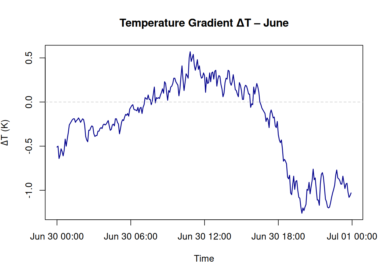
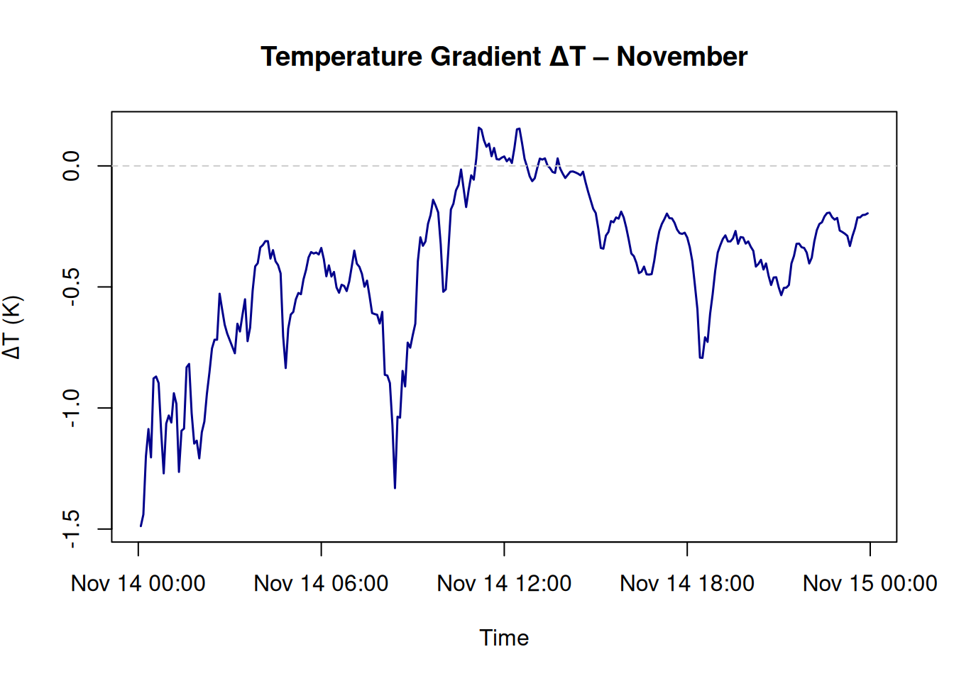
  mutate(
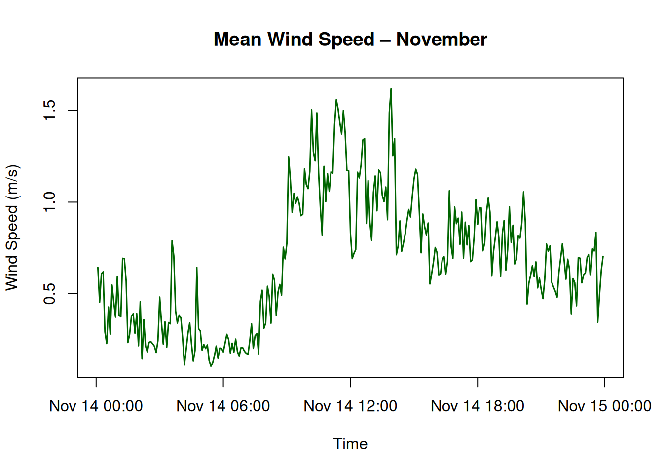
    delta_T = Ta_2m - Ta_10m,
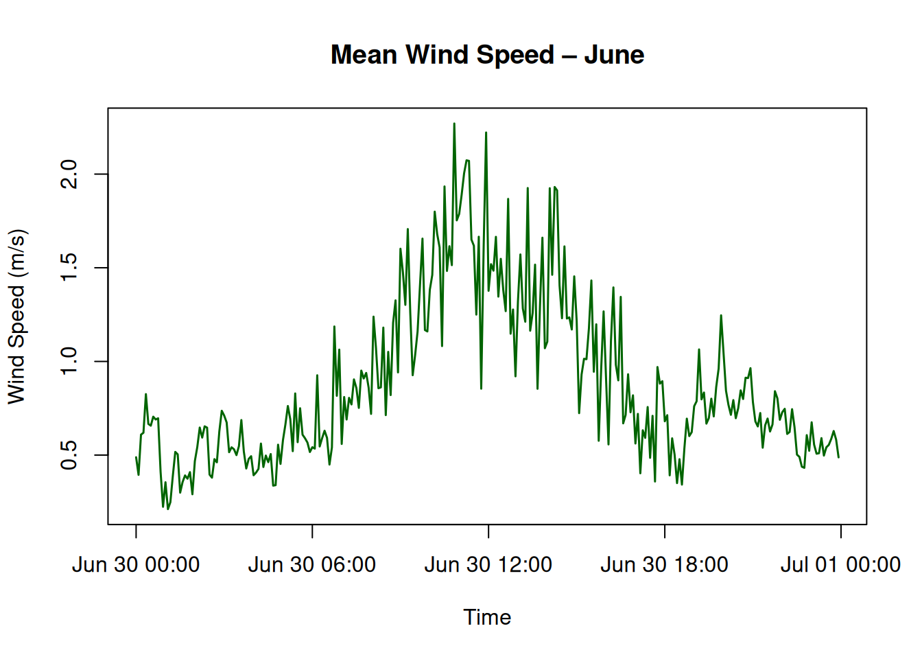
    WS_mean = (WS_2m + WS_10m) / 2,
    month_num = month(datetime),
    month_label = case_when(
      month_num == 6 ~ "June",
      month_num == 11 ~ "November",
      TRUE ~ as.character(month(datetime, label = TRUE))
    )
  )

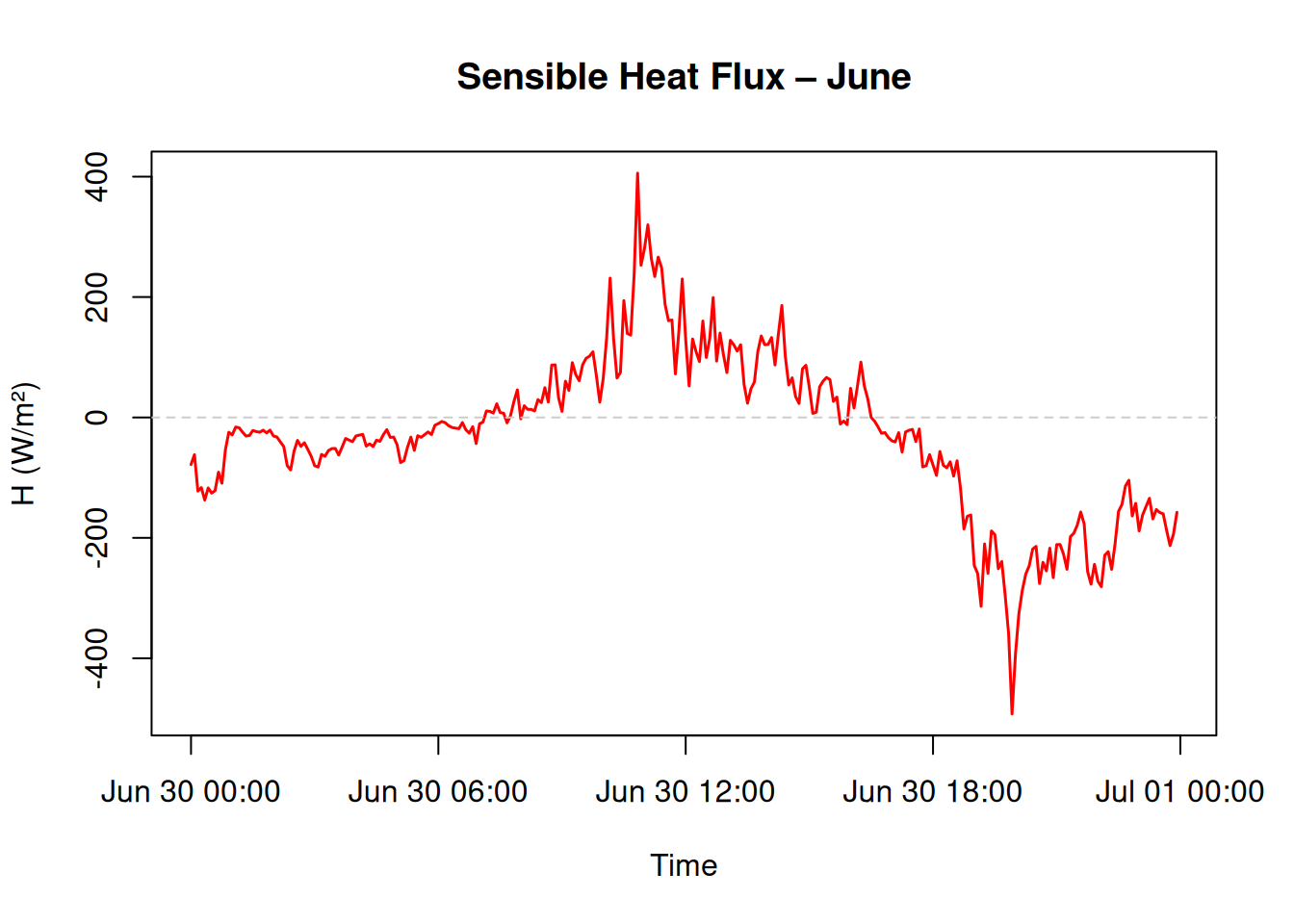
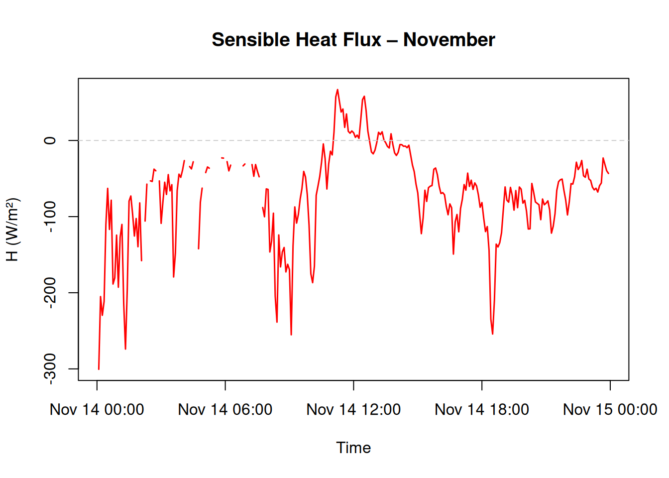
Sensible Heat Flux (H): Bulk Transfer Method

Sensible heat flux (H) is the rate at which thermal energy is transferred from the Earth’s surface to the atmosphere due to a temperature difference. It is a critical term in the surface energy balance and is especially important in meteorology, hydrology, and micrometeorology.

It describes how warm the surface is compared to the air above it — and how turbulent air motion carries that heat away. The bulk transfer formulation for (H) assumes a logarithmic wind profile and neutral atmospheric conditions short explanation adding to the scalar laws.

\[ H = \rho c_p \cdot \frac{\Delta T}{r_a} \]

Where:

Symbol	Meaning
$H$	Sensible heat flux $W/m²$
$rho$	Air density $kg/m³$ (typically ≈ 1.225 at sea level)
$c_p$	Specific heat of air at constant pressure $J/kg/K$ $≈ 1005 J/kg/K$
$Delta T$	Temperature difference between two heights: $T\_{z2} - T\_{z1}$ $K$
$r_a$	Aerodynamic resistance to heat transfer $s/m$

Aerodynamic Resistance $r_a$

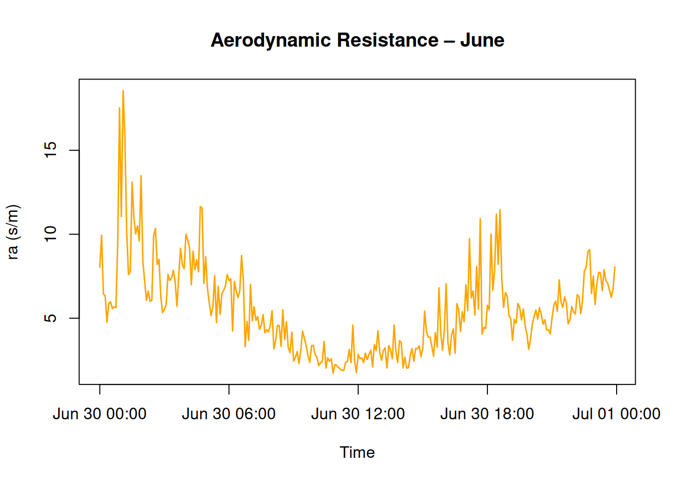
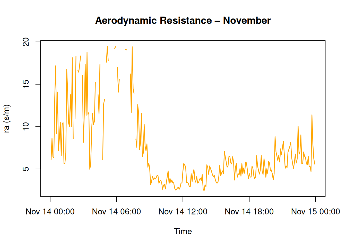
Aerodynamic resistance quantifies how turbulent air mixes heat. It depends on wind speed, measurement height, and surface roughness.

For a flat and open surface, and assuming a neutral atmosphere:

\[r_a = \frac{\ln(z_2/z_1)}{k \cdot u_{mean}}\]

Where:

Symbol	Meaning
$z_1$	Lower measurement height (e.g. 2 m)
$z_2$	Upper measurement height (e.g. 10 m)
$k$	von Kármán constant (≈ 0.41)
$u\_{mean}$	Mean horizontal wind speed between $z_1$ and $z_2$ $m/s$

This formula assumes: - horizontally homogeneous surface, - fully turbulent flow, - negligible atmospheric stability effects (i.e. neutral conditions).

Wind profile, buoyancy effects and turbulent scalar transport

Note on logarithmic wind profile

A logarithmic wind profile means that wind speed increases with height according to:

\[ u(z) = \frac{u_*}{k} \ln\left(\frac{z}{z_0}\right) \]

where $u_*$ is the friction velocity, $k$ the von Kármán constant, and $z_0$ the roughness length. This profile arises from surface-layer theory under turbulent, steady conditions.

Note on Diagnosing Atmospheric Stability

To determine whether neutral atmospheric stratification applies, we estimate the Obukhov length $L$, a key parameter from Monin–Obukhov similarity theory:

\[ L = -\frac{\rho \cdot c_p \cdot T \cdot u_*^3}{k \cdot g \cdot H} \]

where:

$\rho = 1.225\,\text{kg/m}^3$: air density
$c_p = 1005\,\text{J/kg/K}$: specific heat of air
$T$: mean air temperature (in K)
$u_*$: friction velocity (approximated)
$k = 0.41$: von Kármán constant
$g = 9.81\,\text{m/s}^2$: gravitational acceleration
$H$: sensible heat flux (W/m²)

We estimate $u_*$ from wind speed using the log-profile equation:

\[ u_* = \frac{k \cdot \bar{u}}{\ln(z_2 / z_1)} \]

and compute:

$T = (T_{2m} + T_{10m})/2 + 273.15$
$\bar{u} = (u_{2m} + u_{10m}) / 2$

The dimensionless height $z/L$ is then used to classify stability:

$|z/L| < 0.1$ → Neutral
$z/L > 0.1$ → Stable
$z/L < -0.1$ → Unstable

This allows us to screen the dataset and verify whether bulk formulations assuming neutral stratification are valid at given time steps.

Note on Scalar Transport Laws

Turbulent scalar transport refers to the movement of quantities like temperature or humidity due to turbulent eddies in the atmosphere. These fluxes follow a gradient–flux relationship:

\[ F_\phi = -K_\phi \cdot \frac{\partial \phi}{\partial z} \]

where:

$F_\phi$: vertical flux of scalar $\phi$ (e.g. $T$, $q$),
$K_\phi$: eddy diffusivity [m²/s],
$\frac{\partial \phi}{\partial z}$: vertical gradient of the scalar.

In field applications, this is simplified into bulk transfer formulas like:

\[ H = \rho \cdot c_p \cdot \frac{\Delta T}{r_a} \]

which relate scalar differences to vertical fluxes via aerodynamic resistance $r_a$.

Assumptions and Limitations

-   Assumes neutral stability — ignores buoyancy effects (unstable/stable conditions).

-   Requires accurate wind and temperature measurements.

-   Works best over homogeneous, flat terrain.

-   May underestimate or overestimate fluxes under low wind or very moist/dry conditions.

Code

# Constants
rho_air <- set_units(1.225, "kg/m^3")
cp_air <- set_units(1005, "J/kg/K")
z1 <- 2
z2 <- 10
k <- 0.41

energy <- energy %>%
  mutate(
    ra = log(z2 / z1) / (k * WS_mean),
    H = drop_units(rho_air * cp_air * delta_T / ra)
  )

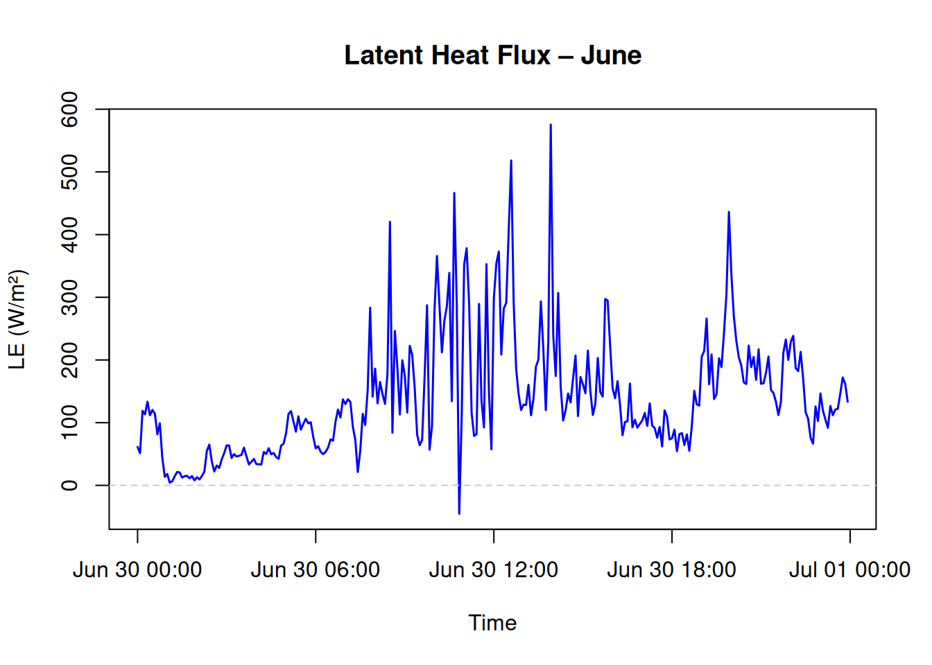
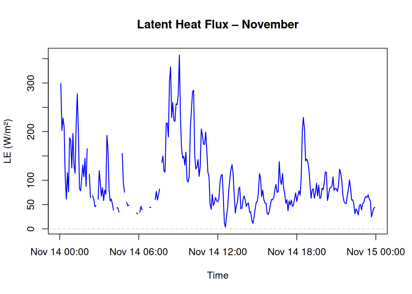
Latent Heat Flux $LE$: Residual Method

The latent heat flux $LE$ quantifies the energy used for evapotranspiration — the combined loss of water to the atmosphere by:

evaporation from soil and wet surfaces,
transpiration through stomata in plants, and
evaporation of intercepted rainfall from canopy surfaces.

Residual Energy Balance Equation

When direct measurement is unavailable, we estimate $LE$ as the residual of the surface energy balance by subtracting all the known energy components from the total incoming energy:

\[ LE = R_n - G - H \]

Where:

$LE$: latent heat flux [W/m²]
$R_n$: net radiation [W/m²] (incoming − outgoing radiation)
$G$: ground heat flux [W/m²] (into or out of the soil)
$H$: sensible heat flux [W/m²] (convective heat to the air)

Assumptions and Cautions

Assumes energy balance closure (no significant storage (S)).
Errors in $R_n$, $G$, or $H$ directly affect $LE$.
Nighttime or low-flux periods often show non-physical negative (LE).

Linking Bulk and Residual Approaches

To estimate the surface energy balance components, we combine two complementary methods:

Sensible heat flux $H$ is derived using the bulk transfer approach, which relies on measured temperature and wind speed differences at two heights.
Latent heat flux $LE$ is then calculated as the residual energy — the portion of net radiation not used for heating the air ($H$) or the soil ($G$).

Component	Bulk Transfer Method	Residual Method
What it estimates	Sensible heat flux ($H$)	Latent heat flux ($LE$)
Required inputs	$\Delta T$ (temp. difference), $\bar{u}$ (mean wind speed)	$R_n$ (net radiation), $G$ (ground heat), and $H$
Physical principle	Turbulent heat transport via scalar gradient	Energy conservation (surface energy balance)
Formula used	$H = \rho \cdot c_p \cdot \dfrac{\Delta T}{r_a}$	$LE = R_n - G - H$
Key assumption	Logarithmic wind profile, neutral stratification	Negligible storage term $S \approx 0$
Output in your case	$H = 251\,\text{W/m}^2$ (based on realistic inputs)	$LE = 289\,\text{W/m}^2$ (by residual)

Step 1: Bulk Estimation of Sensible Heat Flux

We use the following measured or typical values from a grassland site at midday:

$T_{10m} = 19.0^\circ C$
$T_{2m} = 18.5^\circ C$ → $\Delta T = 0.5\,\text{K}$
Wind speeds: $u_{2m} = 1.2\,\text{m/s}$, $u_{10m} = 2.0\,\text{m/s}$ → $\bar{u} = 1.6\,\text{m/s}$
Constants:
- $\rho = 1.225\,\text{kg/m}^3$ (air density)
- $c_p = 1005\,\text{J/kg/K}$ (specific heat of air)
- $k = 0.41$ (von Kármán constant)
- $z_1 = 2\,\text{m}$, $z_2 = 10\,\text{m}$

Aerodynamic resistance is estimated using the logarithmic wind profile assumption:

\[ r_a = \frac{\ln(z_2 / z_1)}{k \cdot \bar{u}} = \frac{\ln(10 / 2)}{0.41 \cdot 1.6} \approx 2.453\,\text{s/m} \]

Now we insert this into the bulk formula for $H$:

\[ H = \rho \cdot c_p \cdot \frac{\Delta T}{r_a} = 1.225 \cdot 1005 \cdot \frac{0.5}{2.453} \approx 251\,\text{W/m}^2 \]

Step 2: Residual Estimation of Latent Heat Flux

We now assume the following additional energy balance terms are available:

$R_n = 620\,\text{W/m}^2$: net radiation (measured via radiometer)
$G = 80\,\text{W/m}^2$: ground heat flux (from soil heat flux plates)

We calculate latent heat flux $LE$ as the residual:

\[ LE = R_n - G - H = 620 - 80 - 251 = 289\,\text{W/m}^2 \]

This gives the amount of energy used for evaporation and transpiration, inferred from energy conservation.

Interpretation

By first estimating $H$ via physical gradients (bulk approach), and then applying the residual method, we close the energy balance without needing direct $LE$ measurements. This is a standard practice in micrometeorology when eddy covariance data are not available.

Using the residual method:

$LE = R_n - G - H$

Code

energy <- energy %>% mutate(LE = Rn - G - H)

Plot: Seasonal Comparison of Energy Fluxes

Code

library(ggplot2)

energy_long <- energy %>%
  select(datetime, month_label, Rn, G, H, LE) %>%
  pivot_longer(cols = c(Rn, G, H, LE), names_to = "flux", values_to = "value")

plot_fluxes <- function(df, title) {
  ggplot(df, aes(x = datetime, y = value, color = flux)) +
    geom_line() +
    labs(title = title, x = "Time", y = "Flux (W/m²)") +
    theme_minimal()
}

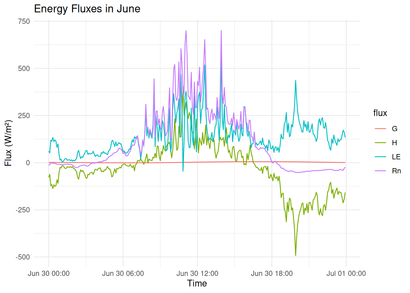
plot_fluxes(filter(energy_long, month_label == "June"), "Energy Fluxes in June")

Energy Fluxes in June

High latent heat flux (LE) dominates, indicating active evapotranspiration.
Sensible heat (H) remains moderate, as much energy is used to vaporize water.
Ground heat flux (G) is positive in early hours, storing heat in the soil.

This matches expectations for early summer (June): longer days, moist soils, and active vegetation cover.

Code

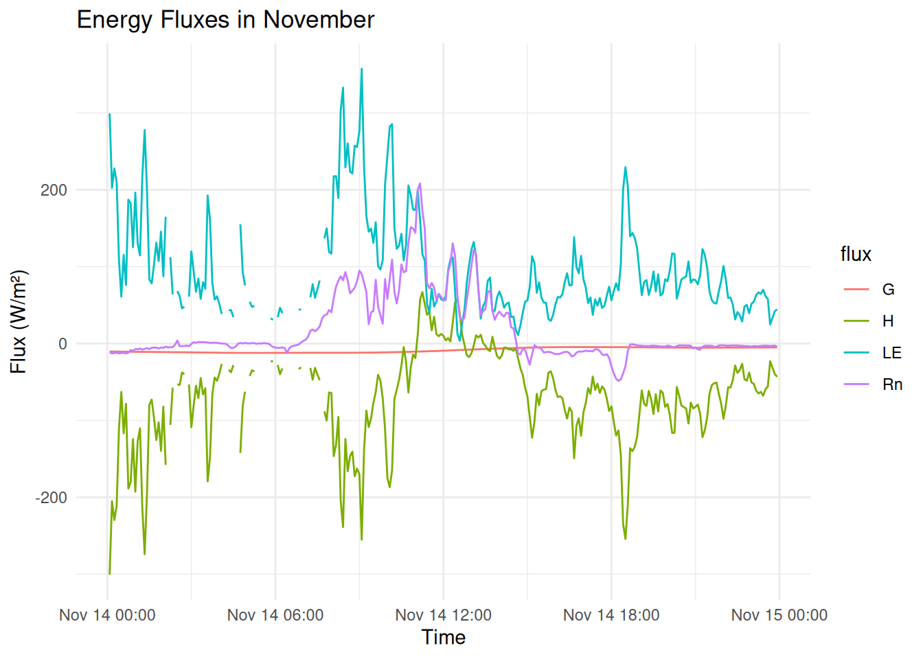
plot_fluxes(filter(energy_long, month_label == "November"), "Energy Fluxes in November")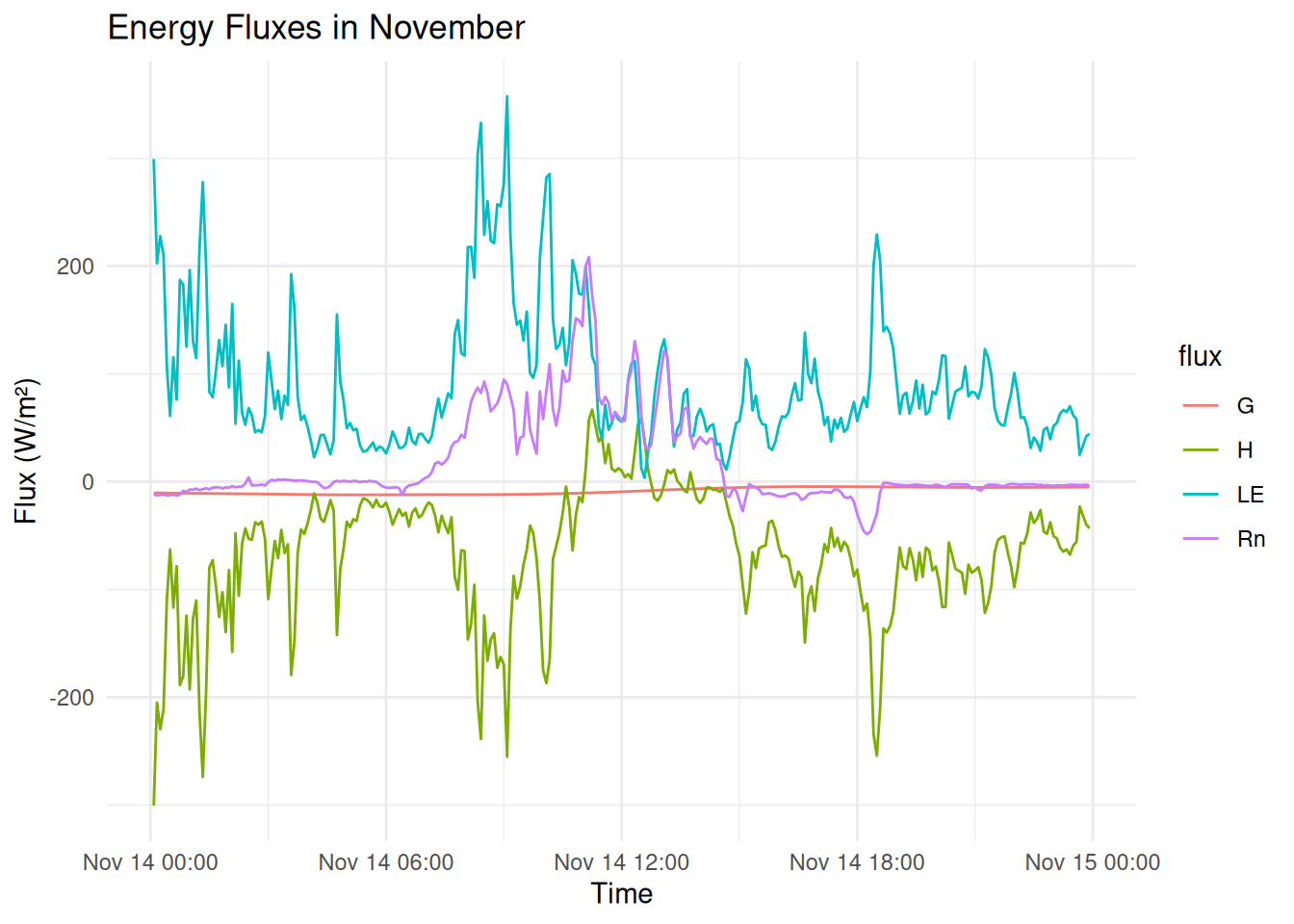

Energy Fluxes in November

Latent heat (LE) is minimal — vegetation is inactive and evapotranspiration drops.
Sensible heat (H) becomes dominant — energy heats the air due to lack of biological water flux.
Ground heat flux (G) may show inversion (soil losing heat), particularly in the evening.

This pattern reflects the dormant season, with minimal biological activity and colder atmospheric conditions.

Legend for Energy Flux Components

Symbol	Description	Sign Convention
(R_n)	Net radiation	Positive downward
(H)	Sensible heat flux	Positive upward (to air)
(LE)	Latent heat flux	Positive upward (evaporation)
(G)	Ground heat flux	Positive downward (into soil)

Notes on Interpretation

Fluxes are sensitive to soil moisture, vegetation, radiation, and wind.
Deviations in (R_n - G - H) often indicate instrument imbalance, storage terms, or closure errors.
The residual approach to compute (LE) assumes high accuracy of the measured and modeled terms.

Convert to Evapotranspiration (mm/day)

We calculate latent heat flux $LE$ as the residual:

\[ LE = R_n - G - H = 620 - 80 - 251 = 289\,\text{W/m}^2 \]

Using latent heat of vaporization $lambda = 2.45 \cdot 10^6\,\text{J/kg}$:

\[ ET = \frac{LE}{\lambda} \cdot \frac{86400}{1000} \]

Insert values:

\[ ET = \frac{330}{2.45 \cdot 10^6} \cdot 86.4 \approx 11.64\,\text{mm/day} \]

On this day, the land surface lost ~11.6 mm of water via evapotranspiration — a very high rate, consistent with moist soil, strong radiation, and active vegetation.

Code

library(dplyr)
library(ggplot2)

# Berechne ET
lambda <- 2.45e6  # J/kg
energy <- energy %>%
  mutate(
    ET_mm_day = (LE / lambda) * 86400,
    month_label = month(datetime, label = TRUE, abbr = FALSE)
  )

# Aggregiere pro Monat
monthly_et <- energy %>%
  filter(!is.na(ET_mm_day)) %>%
  group_by(month_label) %>%
  summarise(
    mean_ET = mean(ET_mm_day, na.rm = TRUE),
    .groups = "drop"
  )

# Plot
ggplot(monthly_et, aes(x = month_label, y = mean_ET, fill = month_label)) +
  geom_col(show.legend = FALSE) +
  labs(
    title = "Mean Daily Evapotranspiration (ET) from Residual Method",
    x = "Month",
    y = "Evapotranspiration (mm/day)"
  ) +
  scale_fill_manual(values = c("June" = "tomato", "November" = "turquoise3")) +
  theme_minimal()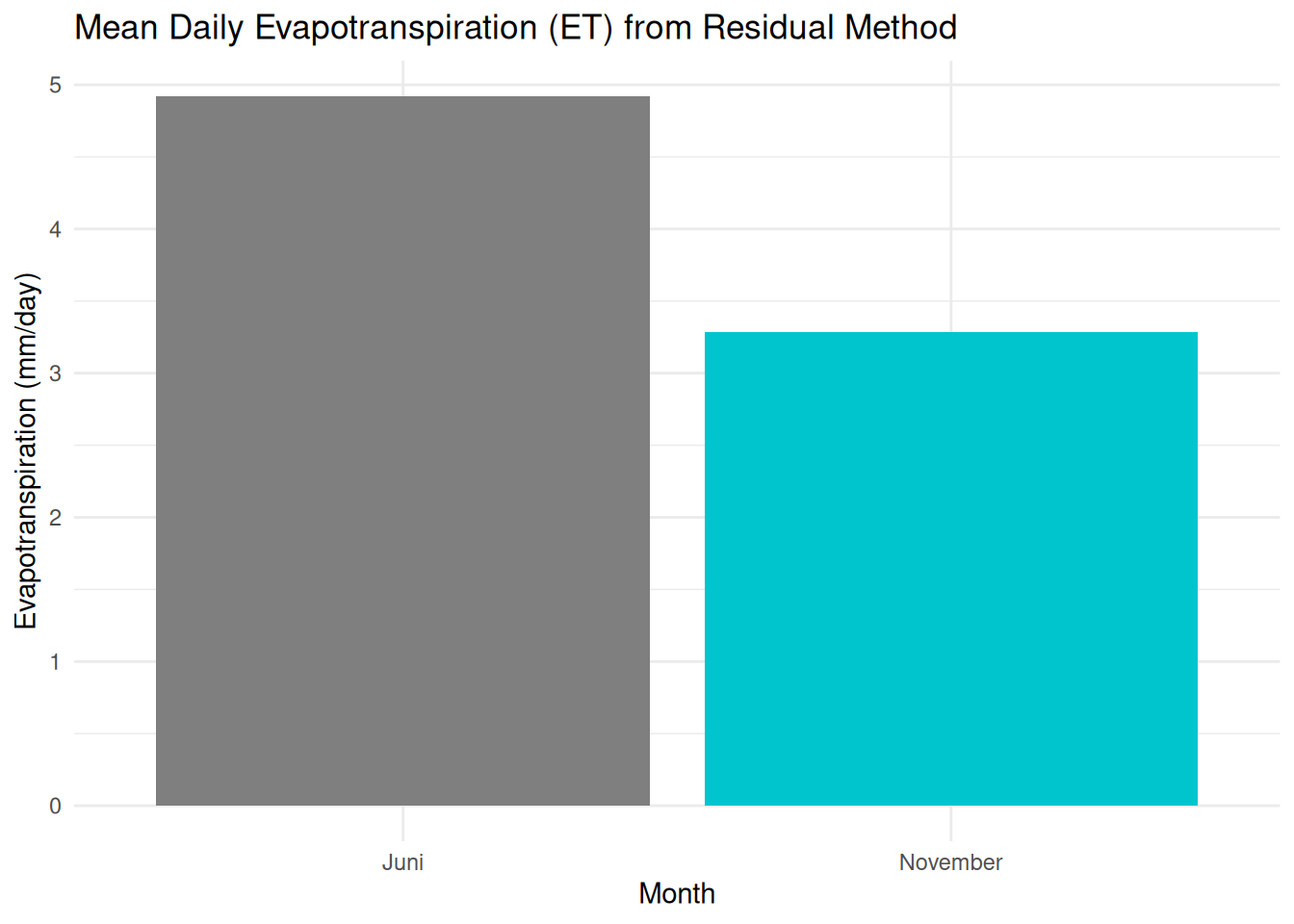

Export (Optional)

Code

# write_csv(energy, here::here("data", "processed_energy_fluxes.csv"))

Complete Code

Code

# Setup: source external script
source("../src/fluxes_corrected.R")

References

Foken, T. (2008). Micrometeorology. Springer.
Monteith, J. L., & Unsworth, M. H. (2013). Principles of Environmental Physics. Academic Press.
Allen, R. G., Pereira, L. S., Raes, D., & Smith, M. (1998). Crop evapotranspiration – FAO Irrigation and Drainage Paper 56.
Arya, S. P. (2001). Introduction to Micrometeorology. Academic Press.
Oke, T. R. (2002). Boundary Layer Climates. Routledge.

Symbol	Meaning
\(H\)	Sensible heat flux \(W/m²\)
\(rho\)	Air density \(kg/m³\) (typically ≈ 1.225 at sea level)
\(c_p\)	Specific heat of air at constant pressure \(J/kg/K\) \(≈ 1005 J/kg/K\)
\(Delta T\)	Temperature difference between two heights: \(T\_{z2} - T\_{z1}\) \(K\)
\(r_a\)	Aerodynamic resistance to heat transfer \(s/m\)

Basic Energy Flux Analysis from Energy Balance Station

Introduction

Surface Energy Balance: Theory and Interpretation

Basic Surface Energy Balance Equation

Load Libraries and Data

Preprocessing

Sensible Heat Flux (H): Bulk Transfer Method

Aerodynamic Resistance \(r_a\)

Note on logarithmic wind profile

Note on Diagnosing Atmospheric Stability

Note on Scalar Transport Laws

Assumptions and Limitations

Latent Heat Flux \(LE\): Residual Method

Residual Energy Balance Equation

Assumptions and Cautions

Linking Bulk and Residual Approaches

Step 1: Bulk Estimation of Sensible Heat Flux

Step 2: Residual Estimation of Latent Heat Flux

Interpretation

Plot: Seasonal Comparison of Energy Fluxes

Energy Fluxes in June

Energy Fluxes in November

Notes on Interpretation

Export (Optional)

Complete Code

References