library(fieldClim)
library(here)

# Kursprojekt: bevorzugt lokale Datei unter data/.
caldern_file <- here::here("data", "caldern_wiese_2017-06-30.csv")

# Fallback: mit fieldClim ausgelieferter Beispieldatensatz.
if (!file.exists(caldern_file)) {
  caldern_file <- system.file(
    "extdata",
    "caldern_wiese_2017-06-30.csv",
    package = "fieldClim"
  )
}

stopifnot(file.exists(caldern_file))

caldern <- read.csv(
  caldern_file,
  na.strings = c("NULL", "NA", "")
)

caldern$datetime <- as.POSIXct(
  caldern$datetime,
  format = "%Y-%m-%d %H:%M:%S",
  tz = "Europe/Berlin"
)
HinweisQuellcode
Der komplette R-Code dieser Lektion wird im gerenderten Dokument sichtbar angezeigt. Zusätzlich steht der extrahierte und ausführlich kommentierte R-Code als Datei bereit: L03_weather_station_objekt_und_basisworkflow.R.
Ziel dieser Kurseinheit
Diese Einheit stellt fieldClim als Arbeitswerkzeug in den Mittelpunkt. Die Theorie ist bekannt, die Datenprüfung ist erfolgt. Jetzt geht es um die eigentliche Paketlogik: Messspalten, Standort, Oberflächenannahmen und Messhöhen werden in ein weather_station-Objekt übersetzt und danach mit Paketfunktionen ausgewertet.
Das Objekt ist der Kern des Workflows. Es sorgt dafür, dass Strahlung, Boden, Feuchte, Druck, Temperatur, Windprofil und Stabilitätsdiagnosen dieselbe Datengrundlage verwenden. Genau hier entsteht die praktische Verbindung zwischen Klimastation und Modellanwendung.
HinweisArbeitsprinzip in R
Der Code bleibt absichtlich einfach. Wir verwenden read.csv(), direkte Spaltenzugriffe mit $, kleine data.frame()-Tabellen und base-R-Plots. Das Ziel ist nicht ein eleganter R-Stil, sondern eine nachvollziehbare Übersetzung von Stationsdaten in fieldClim-Berechnungen. Pfade laufen über here::here(). Wenn die Kursdatei data/caldern_wiese_2017-06-30.csv nicht vorhanden ist, nutzt der Code als Fallback die mit dem Paket ausgelieferte Beispieldatei.
Arbeitsgrößen vorbereiten
Wir übernehmen in dieser Einheit die Arbeitsentscheidung aus der Datenprüfung: rad_net wird als Q_star verwendet und heatflux_soil als B. Die Alternativen aus den Strahlungskomponenten bleiben Diagnosegrößen, aber sie ersetzen nicht still die Messspalte.
caldern$Q_star <- caldern$rad_net
caldern$B <- caldern$heatflux_soil
caldern$A <- caldern$Q_star - caldern$B

summary(caldern[, c("Q_star", "B", "A")])
#>      Q_star             B                  A
#>  Min.   :-52.36   Min.   :-0.75577   Min.   :-56.84
#>  1st Qu.:-17.43   1st Qu.: 0.02899   1st Qu.:-17.75
#>  Median : 48.34   Median : 1.55380   Median : 47.75
#>  Mean   :110.84   Mean   : 2.14723   Mean   :108.69
#>  3rd Qu.:215.55   3rd Qu.: 4.48683   3rd Qu.:210.15
#>  Max.   :700.70   Max.   : 5.59189   Max.   :698.25
Das Stationsobjekt bauen
Der folgende Chunk ist der wichtigste technische Schritt. Er ist bewusst ausgeschrieben. Man soll sehen, welche Messspalte welche Rolle bekommt. Für eine Lehreinheit ist das besser als eine stark verkürzte Hilfsfunktion, weil genau in dieser Zuordnung die meisten fachlichen Fehler entstehen.
ws <- build_weather_station(
  datetime = caldern$datetime,
  lon = 8.6832,
  lat = 50.8405,
  elev = 261,

  temp = caldern$Ta_2m,
  rh = caldern$Huma_2m,

  t1 = caldern$Ta_2m,
  t2 = caldern$Ta_10m,
  hum1 = caldern$Huma_2m,
  hum2 = caldern$Huma_10m,

  v1 = caldern$Windspeed_2m,
  v2 = caldern$Windspeed_10m,
  z1 = 2,
  z2 = 10,

  rad_bal = caldern$rad_net,
  soil_flux = caldern$heatflux_soil,

  slope = 0,
  exposition = 0,
  valley = FALSE,
  surface_type = "field",
  surface_temp = caldern$Ts,

  texture = "peat",
  moisture = caldern$water_vol_soil,
  soil_temp1 = caldern$Ts,
  soil_temp2 = caldern$Ta_2m,
  soil_depth1 = 0.25,
  soil_depth2 = 0,
  obs_height = 2
)class(ws)
#> [1] "weather_station"
names(ws)
#> [1] "datetime" "lon" "lat" "elev" "temp"
#> [6] "rh" "t1" "t2" "hum1" "hum2"
#> [11] "v1" "v2" "z1" "z2" "rad_bal"
#> [16] "soil_flux" "slope" "exposition" "valley" "surface_type"
#> [21] "surface_temp" "texture" "moisture" "soil_temp1" "soil_temp2"
#> [26] "soil_depth1" "soil_depth2" "obs_height"
head(as.data.frame(ws))
#> datetime lon lat elev temp rh t1 t2 hum1 hum2
#> 1 2017-06-30 00:00:00 8.6832 50.8405 261 13.09 100.0 13.09 13.60 100.0 97.6
#> 2 2017-06-30 00:05:00 8.6832 50.8405 261 13.01 100.0 13.01 13.51 100.0 97.7
#> 3 2017-06-30 00:10:00 8.6832 50.8405 261 13.02 100.0 13.02 13.66 100.0 96.5
#> 4 2017-06-30 00:15:00 8.6832 50.8405 261 13.16 100.0 13.16 13.76 100.0 96.1
#> 5 2017-06-30 00:20:00 8.6832 50.8405 261 13.27 100.0 13.27 13.80 100.0 96.4
#> 6 2017-06-30 00:25:00 8.6832 50.8405 261 13.69 98.1 13.69 14.25 98.1 92.4
#> v1 v2 z1 z2 rad_bal soil_flux slope exposition valley surface_type
#> 1 0.448 0.529 2 10 -15.200 1.551533 0 0 FALSE field
#> 2 0.380 0.409 2 10 -8.920 1.492695 0 0 FALSE field
#> 3 0.548 0.670 2 10 -1.965 1.448708 0 0 FALSE field
#> 4 0.581 0.658 2 10 -1.790 1.390439 0 0 FALSE field
#> 5 0.764 0.887 2 10 -2.469 1.325316 0 0 FALSE field
#> 6 0.589 0.744 2 10 -3.857 1.268762 0 0 FALSE field
#> surface_temp texture moisture soil_temp1 soil_temp2 soil_depth1 soil_depth2
#> 1 16.31 peat 0.344 16.31 13.09 0.25 0
#> 2 16.29 peat 0.344 16.29 13.01 0.25 0
#> 3 16.25 peat 0.344 16.25 13.02 0.25 0
#> 4 16.25 peat 0.344 16.25 13.16 0.25 0
#> 5 16.22 peat 0.344 16.22 13.27 0.25 0
#> 6 16.19 peat 0.344 16.19 13.69 0.25 0
#> obs_height
#> 1 2
#> 2 2
#> 3 2
#> 4 2
#> 5 2
#> 6 2Das Objekt trägt zwei Arten von Information. Erstens enthält es Messwerte: Temperatur, Feuchte, Wind, Strahlung, Bodenwärmestrom. Zweitens enthält es Annahmen: Oberflächentyp, Messhöhen, Standort, Hangneigung, Exposition, Bodenart und Beobachtungshöhe. Beide Gruppen sind methodisch relevant.
Eingaben inspizieren
Bevor Wärmeflussmethoden laufen, muss geprüft werden, welche Eingaben vollständig vorhanden sind. inspect_weather_station_inputs() repariert keine Daten. Die Funktion meldet, welche Felder vorhanden sind, wo Lücken liegen und welche Methodenfamilien aus Eingabesicht bereit sind.
inspection <- inspect_weather_station_inputs(ws)

names(inspection)
#> [1] "fields"           "gaps"             "method_readiness" "qc_flags"
#> [5] "guidance"         "summary"
inspection$summary
#> $n_fields
#> [1] 42
#>
#> $n_missing_fields
#> [1] 14
#>
#> $n_partial_fields
#> [1] 0
#>
#> $n_gaps
#> [1] 0
#>
#> $n_qc_flags
#> [1] 0
#>
#> $ready_methods
#> [1] "priestley_taylor"       "bulk_residual"          "bulk_residual_ri_guard"
#> [4] "bowen"                  "monin_profile"          "penman"
#>
#> $blocked_methods
#> character(0)
#>
#> $unsafe_missing_fields
#> character(0)

subset(
  inspection$fields,
  source_status != "present"
)
#>                    field present all_missing any_missing n_missing n_total
#> 6                rad_net   FALSE        TRUE        TRUE         0       0
#> 7              rad_sw_in   FALSE        TRUE        TRUE         0       0
#> 8             rad_sw_out   FALSE        TRUE        TRUE         0       0
#> 9              rad_lw_in   FALSE        TRUE        TRUE         0       0
#> 10            rad_lw_out   FALSE        TRUE        TRUE         0       0
#> 11                albedo   FALSE        TRUE        TRUE         0       0
#> 22          thermal_cond   FALSE        TRUE        TRUE         0       0
#> 28       vapour_pressure   FALSE        TRUE        TRUE         0       0
#> 29        vapor_pressure   FALSE        TRUE        TRUE         0       0
#> 30     absolute_humidity   FALSE        TRUE        TRUE         0       0
#> 31     specific_humidity   FALSE        TRUE        TRUE         0       0
#> 32              pressure   FALSE        TRUE        TRUE         0       0
#> 36 potential_temperature   FALSE        TRUE        TRUE         0       0
#> 39              wind_dir   FALSE        TRUE        TRUE         0       0
#>    missing_fraction source_status     group         variable_type
#> 6                NA       missing radiation             radiation
#> 7                NA       missing radiation             radiation
#> 8                NA       missing radiation             radiation
#> 9                NA       missing radiation             radiation
#> 10               NA       missing radiation             radiation
#> 11               NA       missing radiation             radiation
#> 22               NA       missing      soil soil thermal property
#> 28               NA       missing  humidity              humidity
#> 29               NA       missing  humidity              humidity
#> 30               NA       missing  humidity              humidity
#> 31               NA       missing  humidity              humidity
#> 32               NA       missing  pressure              pressure
#> 36               NA       missing  profiles           temperature
#> 39               NA       missing  profiles        wind direction

inspection$method_readiness[, c(
  "method",
  "missing_fields",
  "partial_fields",
  "ready",
  "notes"
)]
#>                   method missing_fields partial_fields ready
#> 1       priestley_taylor                                TRUE
#> 2          bulk_residual                                TRUE
#> 3 bulk_residual_ri_guard                                TRUE
#> 4                  bowen                                TRUE
#> 5          monin_profile                                TRUE
#> 6                 penman                                TRUE
#>                                                                                                       notes
#> 1 Requires available measured input fields for temperature, net radiation, soil heat flux and surface type.
#> 2                                          Neutral bulk path can use v1 only; v2 is optional for mean wind.
#> 3                         Optional Richardson guard requires v2 and remains unavailable when v2 is missing.
#> 4                                                     Requires two-level temperature and humidity profiles.
#> 5                                           Requires profile inputs plus either surface_type or obs_height.
#> 6                  Uses hum1 when present, otherwise rh; both are interpreted as relative humidity percent.
Die Funktion ist ein Kontrollpunkt, keine Freigabe. Wenn eine Methode „ready“ ist, bedeutet das: Die benötigten Felder sind strukturell vorhanden. Es bedeutet nicht automatisch, dass jeder Zeitschritt meteorologisch gut konditioniert ist. Das wird erst durch Stabilitäts- und Ergebnisdiagnosen sichtbar.
Modellierte Strahlung als Plausibilitätsmaßstab
fieldClim enthält Funktionen, um Strahlung aus Zeit, Standort, Gelände und Oberflächenannahmen zu modellieren. In dieser Kurseinheit wird das nicht als Ersatzmessung eingeführt. Modellierte Strahlung ist hier ein Plausibilitätsmaßstab: Stimmen Tagesgang und Größenordnung ungefähr, oder deutet etwas auf Zeitzone, Spaltendefinition oder falsche Annahmen hin?
lon <- 8.6832
lat <- 50.8405
elev <- 261
slope <- 0
exposition <- 0
valley <- FALSE
surface_type <- "field"

caldern$K_down_model <- rad_sw_in(
  caldern$datetime,
  lon, lat, elev, caldern$Ta_2m,
  slope, exposition
)

caldern$Q_star_model <- rad_bal(
  caldern$datetime, lon, lat, elev,
  caldern$Ta_2m, caldern$Huma_2m,
  slope, exposition, valley, surface_type,
  caldern$Ts
)

summary(caldern[, c("rad_sw_in", "K_down_model", "rad_net", "Q_star_model")])
#>    rad_sw_in          K_down_model      rad_net        Q_star_model
#>  Min.   :  -2.0210   Min.   :  0.0   Min.   :-52.36   Min.   :-117.2
#>  1st Qu.:  -0.2645   1st Qu.:  0.0   1st Qu.:-17.43   1st Qu.:-105.5
#>  Median :  89.5500   Median :187.4   Median : 48.34   Median : 102.0
#>  Mean   : 189.1081   Mean   :269.0   Mean   :110.84   Mean   : 162.8
#>  3rd Qu.: 342.2500   3rd Qu.:536.9   3rd Qu.:215.55   3rd Qu.: 433.9
#>  Max.   :1003.0000   Max.   :703.3   Max.   :700.70   Max.   : 569.6
op <- par(mfrow = c(2, 1), mar = c(3.5, 4, 2, 1))
plot(caldern$datetime, caldern$rad_sw_in, type = "l",
xlab = "Zeit", ylab = "W m-2", main = "Kurzwellige Einstrahlung")
lines(caldern$datetime, caldern$K_down_model, lty = 2)
legend("topright", legend = c("gemessen", "modelliert"),
lty = c(1, 2), bty = "n")
plot(caldern$datetime, caldern$rad_net, type = "l",
xlab = "Zeit", ylab = "W m-2", main = "Netto-Strahlung")
lines(caldern$datetime, caldern$Q_star_model, lty = 2)
legend("bottomleft", legend = c("gemessen", "modelliert"),
lty = c(1, 2), bty = "n")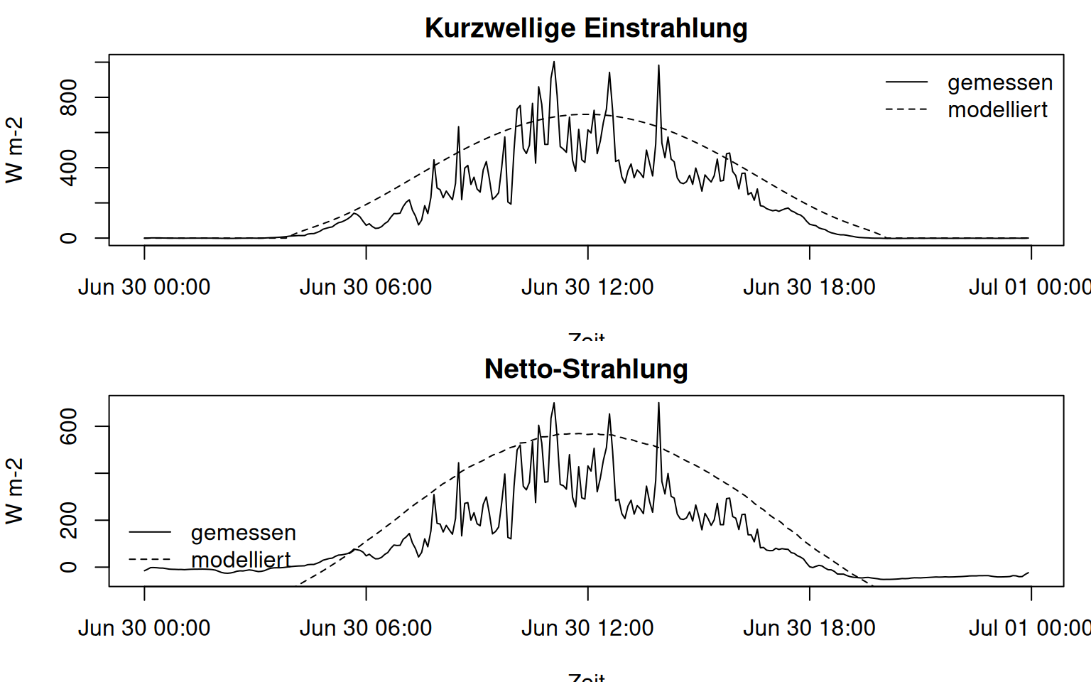
par(op)Die modellierte Reihe muss nicht deckungsgleich mit der Messreihe sein. Sie hilft aber, offensichtliche Probleme zu finden. Ein falscher Zeitzonenbezug verschiebt den Tagesgang. Eine falsche Oberflächenannahme verändert langwellige Ausstrahlung und Bilanz. Eine stark abweichende Größenordnung verlangt eine Prüfung der Sensor- oder Spaltendefinition.
Hilfsgrößen: Feuchte, Dichte, Temperatur
Viele fieldClim-Funktionen erzeugen Größen, die nicht als Endergebnis gedacht sind. Absolute Feuchte, potentielle Temperatur, Luftdichte oder Verdampfungswärme sind Zwischenübersetzungen. Sie verbinden Stationsspalten mit späteren Wärmeflussmethoden.
caldern$hum_abs <- hum_absolute(caldern$Huma_2m, caldern$Ta_2m)
caldern$evap_heat <- hum_evap_heat(caldern$Ta_2m)
caldern$hum_gradient <- hum_moisture_gradient(
  caldern$Huma_2m,
  caldern$Huma_10m,
  caldern$Ta_2m,
  caldern$Ta_10m,
  2, 10, 261
)
caldern$air_density <- pres_air_density(261, caldern$Ta_2m)
caldern$theta <- temp_pot_temp(caldern$Ta_2m, 261)

summary(caldern[, c("hum_abs", "evap_heat", "hum_gradient", "air_density", "theta")])
#>     hum_abs           evap_heat        hum_gradient         air_density
#>  Min.   :0.009325   Min.   :2453052   Min.   :-1.384e-04   Min.   :1.168
#>  1st Qu.:0.010098   1st Qu.:2456082   1st Qu.:-5.213e-05   1st Qu.:1.172
#>  Median :0.010462   Median :2464544   Median :-3.834e-05   Median :1.187
#>  Mean   :0.010676   Mean   :2463389   Mean   :-3.671e-05   Mean   :1.185
#>  3rd Qu.:0.011350   3rd Qu.:2469324   3rd Qu.:-2.394e-05   3rd Qu.:1.195
#>  Max.   :0.011986   Max.   :2472146   Max.   : 1.735e-05   Max.   :1.199
#>      theta
#>  Min.   :13.56
#>  1st Qu.:14.75
#>  Median :16.75
#>  Mean   :17.24
#>  3rd Qu.:20.31
#>  Max.   :21.58
op <- par(mfrow = c(2, 1), mar = c(3.5, 4, 2, 1))
plot(caldern$datetime, caldern$hum_abs, type = "l",
xlab = "Zeit", ylab = "", main = "Absolute Feuchte")
plot(caldern$datetime, caldern$air_density, type = "l",
xlab = "Zeit", ylab = "kg m-3", main = "Luftdichte")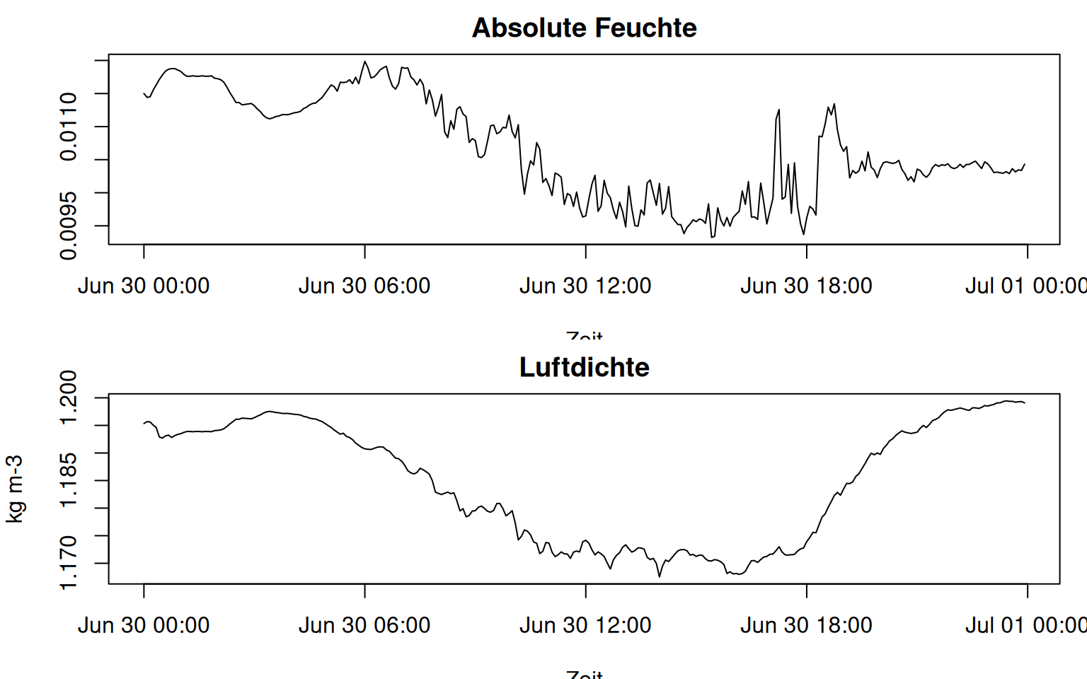
par(op)Die Zwischenvariablen werden nicht isoliert interpretiert. Ihr Wert liegt darin, dass sie spätere Methoden stabiler nachvollziehbar machen. Wenn eine Hilfsgröße falsch skaliert oder lückenhaft ist, taucht das später als scheinbar merkwürdiger Wärmefluss auf.
Windprofil und Stabilität
Profilmethoden reagieren empfindlich auf Temperaturunterschiede, Feuchteunterschiede, Windgeschwindigkeit und Messhöhen. Deshalb werden Windprofil und Stabilität vor der Methodenrechnung geprüft.
z0 <- turb_roughness_length("field")
z0
#> [1] 0.02

caldern$u_star <- turb_ustar(caldern$Windspeed_2m, 2, surface_type = "field")

caldern$richardson <- turb_flux_grad_rich_no(
  caldern$Ta_2m,
  caldern$Ta_10m,
  2,
  10,
  caldern$Windspeed_2m,
  caldern$Windspeed_10m,
  261
)

caldern$exchange_temp <- turb_flux_ex_quotient_temp(
  caldern$Ta_2m,
  caldern$Ta_10m,
  2,
  10,
  caldern$Windspeed_2m,
  caldern$Windspeed_10m,
  261,
  "field"
)

summary(caldern[, c("u_star", "richardson", "exchange_temp")])
#>      u_star          richardson        exchange_temp
#>  Min.   :0.01216   Min.   :-2389.420   Min.   : 0.007292
#>  1st Qu.:0.04271   1st Qu.:   -0.398   1st Qu.: 0.020282
#>  Median :0.05959   Median :    1.346   Median : 0.029678
#>  Mean   :0.06898   Mean   :  265.130   Mean   : 0.301201
#>  3rd Qu.:0.09205   3rd Qu.:    7.225   3rd Qu.: 0.259571
#>  Max.   :0.16998   Max.   :67806.240   Max.   :14.292973
op <- par(mfrow = c(3, 1), mar = c(3.5, 4, 2, 1))
plot(caldern$datetime, caldern$u_star, type = "l",
xlab = "Zeit", ylab = "m s-1", main = "u*: Schubspannungsgeschwindigkeit")
plot(caldern$datetime, caldern$richardson, type = "l",
xlab = "Zeit", ylab = "Ri", main = "Gradient-Richardson-Zahl")
abline(h = 0, lty = 2, col = "grey50")
plot(caldern$datetime, caldern$exchange_temp, type = "l",
xlab = "Zeit", ylab = "", main = "Austauschdiagnose Temperatur")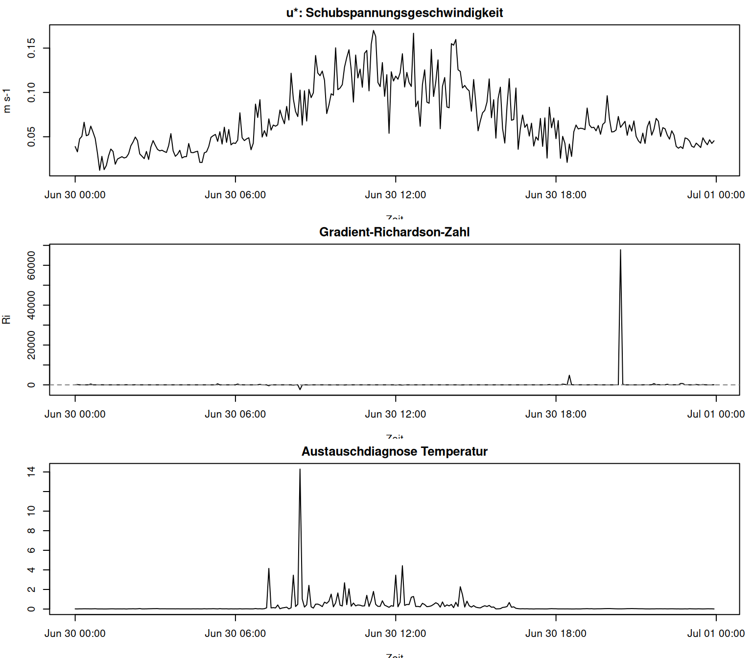
par(op)Diese Werte sind Screeninggrößen. Sie sagen, ob eine Profilauswertung plausibel konditioniert ist. Wenn Windunterschiede sehr klein sind oder die Stabilität stark wechselt, werden spätere Profilflüsse empfindlich. Das ist kein Grund, die Werte zu verstecken. Es ist ein Grund, sie als Diagnose zu lesen.
Objekt ausgeben und plotten
Nach einer Beispielrechnung enthält das Objekt zusätzliche Felder. Für den Einstieg reicht es, das Objekt in eine Tabelle umzuwandeln und einzelne Zeitreihen mit base R zu plotten.
ws_pt <- turb_flux_calc(ws, pt_only = TRUE)
ws_table <- as.data.frame(ws_pt)

names(ws_table)
#>  [1] "datetime"                  "lon"
#>  [3] "lat"                       "elev"
#>  [5] "temp"                      "rh"
#>  [7] "t1"                        "t2"
#>  [9] "hum1"                      "hum2"
#> [11] "v1"                        "v2"
#> [13] "z1"                        "z2"
#> [15] "rad_bal"                   "soil_flux"
#> [17] "slope"                     "exposition"
#> [19] "valley"                    "surface_type"
#> [21] "surface_temp"              "texture"
#> [23] "moisture"                  "soil_temp1"
#> [25] "soil_temp2"                "soil_depth1"
#> [27] "soil_depth2"               "obs_height"
#> [29] "sensible_priestley_taylor" "latent_priestley_taylor"
head(ws_table)
#>              datetime    lon     lat elev  temp    rh    t1    t2  hum1 hum2
#> 1 2017-06-30 00:00:00 8.6832 50.8405  261 13.09 100.0 13.09 13.60 100.0 97.6
#> 2 2017-06-30 00:05:00 8.6832 50.8405  261 13.01 100.0 13.01 13.51 100.0 97.7
#> 3 2017-06-30 00:10:00 8.6832 50.8405  261 13.02 100.0 13.02 13.66 100.0 96.5
#> 4 2017-06-30 00:15:00 8.6832 50.8405  261 13.16 100.0 13.16 13.76 100.0 96.1
#> 5 2017-06-30 00:20:00 8.6832 50.8405  261 13.27 100.0 13.27 13.80 100.0 96.4
#> 6 2017-06-30 00:25:00 8.6832 50.8405  261 13.69  98.1 13.69 14.25  98.1 92.4
#>      v1    v2 z1 z2 rad_bal soil_flux slope exposition valley surface_type
#> 1 0.448 0.529  2 10 -15.200  1.551533     0          0  FALSE        field
#> 2 0.380 0.409  2 10  -8.920  1.492695     0          0  FALSE        field
#> 3 0.548 0.670  2 10  -1.965  1.448708     0          0  FALSE        field
#> 4 0.581 0.658  2 10  -1.790  1.390439     0          0  FALSE        field
#> 5 0.764 0.887  2 10  -2.469  1.325316     0          0  FALSE        field
#> 6 0.589 0.744  2 10  -3.857  1.268762     0          0  FALSE        field
#>   surface_temp texture moisture soil_temp1 soil_temp2 soil_depth1 soil_depth2
#> 1        16.31    peat    0.344      16.31      13.09        0.25           0
#> 2        16.29    peat    0.344      16.29      13.01        0.25           0
#> 3        16.25    peat    0.344      16.25      13.02        0.25           0
#> 4        16.25    peat    0.344      16.25      13.16        0.25           0
#> 5        16.22    peat    0.344      16.22      13.27        0.25           0
#> 6        16.19    peat    0.344      16.19      13.69        0.25           0
#>   obs_height sensible_priestley_taylor latent_priestley_taylor
#> 1          2                 -5.301183              -11.450350
#> 2          2                 -3.308925               -7.103770
#> 3          2                 -1.084238               -2.329470
#> 4          2                 -1.002820               -2.177619
#> 5          2                 -1.189538               -2.604778
#> 6 2 -1.571959 -3.553803plot(ws_table$datetime, ws_table$temp, type = "l",
xlab = "Zeit", ylab = "°C", main = "Temperatur aus dem weather_station-Objekt")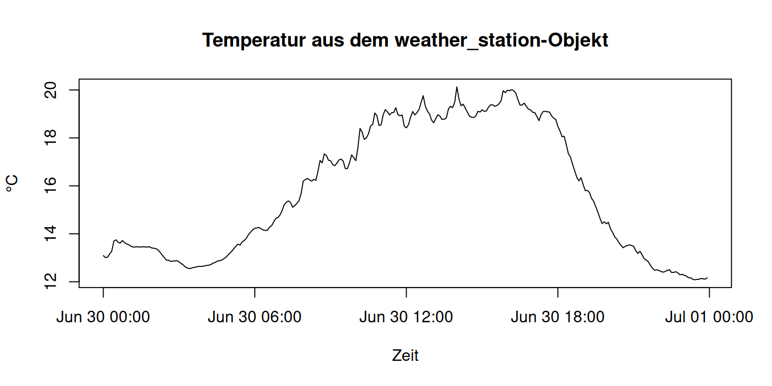
TippArbeitsauftrag
#| echo: true
source(“../assets/scripts/read_cr1000_to_fieldclim.R”)
ws <- read_cr1000_to_fieldclim( file = “../data/myCampbellfile #CR1000_Table1_26Mar.dat”, lon = -0, # Stations-Lon ersetzen lat = -0, # Stations-Lat ersetzen elev = 0, # Stations-Höhe ersetzen tz = “America/Guayaquil”, z1 = 2, z2 = 10, surface_type = “field”, rad_bal_sign = 1, soil_flux_sign = 1 )
class(ws) names(ws)
fieldClim::inspect_weather_station_inputs(ws)
Ändern Sie kontrolliert eine Objektannahme, zum Beispiel surface_type oder obs_height, und bauen Sie das Objekt neu. Prüfen Sie anschließend, welche Folgefunktionen andere Ergebnisse liefern. Dokumentieren Sie nicht nur den Zahlenunterschied, sondern welche fachliche Annahme dahintersteht.