Deriving a CHM from LiDAR & more
Light detection and ranging (LiDAR) observations are point clouds representing the returns of laser pulses reflected from objects, e.g. a tree canopy. Processing LiDAR (or optical point cloud) data generally requires more computational resources than 2D optical observations. The spotlit provides both technical handling of LiDAR data as well as some helpful hints how to optimize the technical and conceptual workflow of programming, data handling and information gathering.
Introduction
LiDAR data and LAS data format
Technically spoken the LiDAR data comes in the LAS file format (for a format definition i.e. have a look at the American Society for Photogrammetry & Remote Sensing LAS documentation file). One LAS data set typically but not necessarily covers an area of 1 km by 1 km. Since the point clouds in the LAS data sets are large, a spatial index file (LAX) considerably reduces search and select operations in the data.
Brief Overview of LiDAR Software Tools
The development of the software is rapid. A few years ago, it was only possible to manipulate, manage and analyze LiDAR data with complex special tools. Especially the (partly (commercial) LAStools software was unrivaled for many years. Many remote sensing and remote sensing software tools have acquired licenses on this basis or developed components independently. Examples are GRASS GIS and ArcGIS. Beside the GIS packages there are a number of powerful specialists. Two important and typical representatives are 3D forest and FUSION.
However all solution can be linked to R (we did it over the years) the lidr package has revolutionized the processing of LiDAR data in the R ecotop and is definitely by far the best choice (and even faster an more reliable than commercial tools). Extensive documentation and workflow examples can be found in the Wiki of the respective GitHub repository. A very recent publication is avaiblable at Remote Sensing of Environment idR: An R package for analysis of Airborne Laser Scanning (ALS) data.
Start up test
For the following, make sure these libraries are part of your setup (should be the case if you follow extended setup spotlight.
We make a short general check that we can start over i.e. if everything is ready to use. First load the tutorial data to an appropriate data folder of your project.
libs = c("lidR", "link2GI", "mapview", "raster", "rgdal", "rlas", "sp", "sf")
# NOTE file size is about 12MB
utils::download.file(url="https://github.com/gisma/gismaData/raw/master/uavRst/data/lidR_data.zip",
                     destfile=paste0(envrmt$path_tmp,"chm.zip"))
unzip(paste0(envrmt$path_tmp,"chm.zip"),
      exdir = envrmt$path_tmp,
      overwrite = TRUE)

las_files = list.files(envrmt$path_tmp,
                       pattern = glob2rx("*.las"),
                       full.names = TRUE)
If you want to read a single (not to big) LAS file, you can use the readLAS function. Plotting the data set results in a 3D interactive screen which opens from within R.
lidar_file = readLAS(las_files[1])
plot(lidar_file, bg = "green", color = "Z",colorPalette = mvTop(256),backend="pcv")
If this works, you’re good to go.
How to get started?
For this first example we take a typical situation:
- we have no idea about the software and possible solutions
- we have no idea about LiDAR data processing and analysis
- we just google something like lidR package tutorial
Among the top ten is The lidR package book. So let’s follow the white rabbit…
Creating a Canopy Height Model (CHM) reloaded
After successful application of the tutorial we will transfer it into a suitable script for our workflow. Please check the comments for better understanding and do it step by step! again. Please note that the following script is meant to be an basic example how:
- to organize scripts in common
- with a hands on example for creating a canopy height model.
After revisiting the tutorial is seems to be a good choice to follow the tutorial of the lidR developer that is Digital Surface Model and Canopy Height model in the above tutorial. Why? because for the first Jean-Romain Roussel explains 6 ways how to create in a very simple approach a CHM, second to show up that it makes sense to read and third to loop back because it does not work with bigger files. Let us start with the new script structure.
#------------------------------------------------------------------------------
# Name: make_CHM_Tiles.R
# Type: control script
# Author: Chris Reudenbach, creuden@gmail.com
# Description:  script creates a canopy height model from generic Lidar
#              las data using the lidR package
# Data: regular las LiDAR data sets
# Copyright: Chris Reudenbach, Thomas Nauss 2017,2019, GPL (>= 3)
#------------------------------------------------------------------------------


# 0 - load packages
#-----------------------------
library("lidR")
library("future")


# 1 - source files
#-----------------

#---- source setup file
source(file.path(envimaR::alternativeEnvi(root_folder = "~/edu/mpg-envinsys-plygrnd",
                                          alt_env_id = "COMPUTERNAME",
                                          alt_env_value = "PCRZP",
                                          alt_env_root_folder = "F:/BEN/edu"),
                 "src/mpg_course_basic_setup.R"))


# 2 - define variables
#---------------------

## define current projection (It is not magic you need to check the meta data or ask your instructor)
## ETRS89 / UTM zone 32N
proj4 = "+proj=utm +zone=32 +datum=WGS84 +units=m +no_defs +ellps=WGS84 +towgs84=0,0,0"


## get viridris color palette
pal<-mapview::mapviewPalette("mapviewTopoColors")

# 3 - start code
#-----------------


 #---- NOTE file size is about 12MB
 utils::download.file(url="https://github.com/gisma/gismaData/raw/master/uavRst/data/lidR_data.zip",
                     destfile=paste0(envrmt$path_tmp,"chm.zip"))
 unzip(paste0(envrmt$path_tmp,"chm.zip"),
      exdir = envrmt$path_tmp,
      overwrite = TRUE)

 #---- Get all *.las files of a folder into a list
 las_files = list.files(envrmt$path_tmp,
                       pattern = glob2rx("*.las"),
                       full.names = TRUE)

 #---- create CHM as provided by
 # https://github.com/Jean-Romain/lidR/wiki/Rasterizing-perfect-canopy-height-models
 las = readLAS(las_files[1])
 las = lidR::lasnormalize(las, knnidw())

 # reassign the projection
 sp::proj4string(las) <- sp::CRS(proj4)

 # calculate the chm with the pitfree algorithm
 chm = lidR::grid_canopy(las, 0.25, pitfree(c(0,2,5,10,15), c(0,1), subcircle = 0.2))

 # write it to tif
 raster::writeRaster(chm,file.path(envrmt$path_data_mof,"mof_chm_one_tile.tif"),overwrite=TRUE)


# 4 - visualize
-------------------

# call mapview with some additional arguments
mapview(raster::raster(file.path(envrmt$path_data_mof,"mof_chm_one_tile.tif")),
         legend=TRUE,
         layer.name = "canopy height model",
         col = pal(256),
         alpha.regions = 0.7)
Full screen version of the map
Coping with computer memory resources
The above example is based on a las-tile of 250 by 250 meter. That means a fairly small tile size. If you did not run in memory or CPU problems you can deal with these tiles by simple looping.
But you have to keep in mind that even if a tile based processing can easily be handled with loops but has some pitfalls. E.g. if you compute some focal operations, you have to make sure that if the filter is close to the boundary of the tile that data from the neighboring tile is loaded in addition. Also the tile size may be a problem for your memory availability.
The lidR package comes with a feature called catalog and a set of catalog functions which make tile-based life easier. A catalog meta object also holds information on e.g. the cartographic reference system of the data or the cores used for parallel processing. So we start over again - this time with a real data set.
If not already done download the course related LiDAR data set of the MOF area. Store the the data to the envrmt$path_lidar_org folder.
Please note that dealing with lidR catalogs is pretty stressful for the memory administration of your rsession. So best practices is to:
- clean the environment
- restart your rsession
This will help you to avoid frustrating situation like restarting your PC after hours of waiting…
#------------------------------------------------------------------------------
# Type: control script
# Name: make_CHM_Catalog.R
# Author: Chris Reudenbach, creuden@gmail.com
# Description:  script creates a canopy height model from generic Lidar
#              las data using the lidR package. In addition the script cuts the area to
#              a defined extent using the lidR catalog concept.
#              Furthermore the data is tiled into a handy format even for poor memory
#              and a canopy height model is calculated
# Data: regular las LiDAR data sets
# Output: Canopy heightmodel RDS file of the resulting catalog
# Copyright: Chris Reudenbach, Thomas Nauss 2017,2020, GPL (>= 3)
#------------------------------------------------------------------------------

## clean your environment
rm(list=ls())

# 0 - load packages
#-----------------------------

library("future")

## dealing with the crs warnings is cumbersome and complex
## you may reduce the warnings with uncommenting  the following line
## for a deeper  however rarely less confusing understanding have a look at:
## https://rgdal.r-forge.r-project.org/articles/CRS_projections_transformations.html
## https://www.r-spatial.org/r/2020/03/17/wkt.html
rgdal::set_thin_PROJ6_warnings(TRUE)


# 1 - source files
#-----------------
source(file.path(envimaR::alternativeEnvi(root_folder = "~/edu/mpg-envinsys-plygrnd",
                                          alt_env_id = "COMPUTERNAME",
                                          alt_env_value = "PCRZP",
                                          alt_env_root_folder = "F:/BEN/edu/mpg-envinsys-plygrnd"),
                 "src/000_setup.R"))


# 2 - define variables
#---------------------

## define current projection (It is not magic you need to check the meta data
## or ask your instructor)
## ETRS89 / UTM zone 32N
## the definition of proj4 strings is kind ob obsolet have a look at the links under section zero
epsg_number = 25832

# switch if lasclip is called
lasclip = FALSE
set.seed(1000)

#  area of interest (central MOF)
xmin = 476174.
ymin = 5631386.
xmax = 478217.
ymax = 5632894.

# test area so called "sap flow halfmoon"
xmin = 477500
ymin = 5631730
xmax = 478350
ymax = 5632500

# define variables for the lidR catalog
chunksize = 250
overlap = 25


# get viridris color palette
pal<-mapview::mapviewPalette("mapviewTopoColors")

# 3 - start code
#-----------------

#---- this part is for clipping only
if (lasclip){
# Get all *.las files of a the folder you have specified to contain the original las files
las_files = list.files(envrmt$path_lidar_org, pattern = glob2rx("*.las"), full.names = TRUE)


#---- NOTE OTIONALLY you can cut the original big data set  to the smaller extent of the MOF
# https://www.rdocumentation.org/packages/lidR/versions/1.6.1/topics/lasclip
core_aoimof<- lidR::lasclipRectangle(lidR::readLAS(las_files[1]), xleft = xmin, ybottom = ymin, xright = xmax, ytop = ymax)

# write the new dataset to the level0 folder and create a corresponding index file (lax)
lidR::writeLAS(core_aoimof,file.path(envrmt$path_level0,"las_mof.las"))
rlas::writelax(file.path(envrmt$path_level0, "las_mof.las"))
} #---- OPTIONAL clipping section finished


#---- We assume that you have the "las_mof.las" file in the folder
#     that is stored in envrmt$path_level0
# setting up a lidR catalog structure
mof100_ctg <- lidR::readLAScatalog(envrmt$path_level0)
projection(mof100_ctg) <- epsg_number
lidR::opt_chunk_size(mof100_ctg) = chunksize
future::plan(multisession)
lidR::opt_chunk_buffer(mof100_ctg) <- overlap
lidR::opt_output_files(mof100_ctg) <- paste0(envrmt$path_normalized,"/{ID}_norm") # add output filname template
mof100_ctg@output_options$drivers$Raster$param$overwrite <- TRUE

#---- derive DTM DEM and CHM information from an ALS point cloud

# the fastest and simplest algorithm to interpolate a surface is given with p2r()
# the available options are  p2r, dsmtin, pitfree
dsm_p2r_1m = grid_canopy(mof100_ctg, res = 1, algorithm = p2r())
plot(dsm_p2r_1m)

# now we calculate a digital terrain model by interpolating the ground points
# and creates a rasterized digital terrain model. The algorithm uses the points
# classified as "ground" and "water (Classification = 2 and 9 according to LAS file format
# available algorithms are  knnidw, tin, and kriging
dtm_knnidw_1m <- grid_terrain(mof100_ctg, res=1, algorithm = knnidw(k = 6L, p = 2))
plot(dtm_knnidw_1m)

# we remove the elevation of the surface from the catalog data and create a new catalog
mof100_ctg_chm <- lidR::normalize_height(mof100_ctg, dtm_knnidw_1m)

# if you want to save this catalog  an reread it  you need
# to uncomment the following lines
#- saveRDS(mof100_ctg_chm,file= file.path(envrmt$path_level1,"mof100_ctg_chm.rds"))
#- mof100_ctg_chm<-readRDS(file.path(envrmt$path_level1,"mof100_ctg_chm.rds"))


# Now create a CHM based on the normalized data and a CHM with the dsmtin() algorithm
# Note the DSM (digital surface model) is now a CHM because we
# already have normalized the data

# first set a NEW  output name for the catalog
lidR::opt_output_files(mof100_ctg_chm) <- paste0(envrmt$path_normalized,"/{ID}_chm_dsmtin") # add output filname template

# calculate a chm raster with dsmtin()/p2r
chm_dsmtin_1m = grid_canopy(mof100_ctg_chm, res=1.0, dsmtin())

# write it to a tif file
raster::writeRaster(chm_dsmtin_1m,file.path(envrmt$path_data_mof,"chm_dsmtin_1m.tif"),overwrite=TRUE)

# 4 - visualize
# -------------------

## standard plot command

plot(raster::raster(file.path(envrmt$path_data_mof,"chm_dsmtin_1m.tif")))

## call mapview with some additional arguments
mapview(raster(file.path(envrmt$path_data_mof,"chm_dsmtin_1m.tif")),
        map.types = "Esri.WorldImagery",
        legend=TRUE,
        layer.name = "canopy height model",
        col = pal(256),
        alpha.regions = 0.65)
The visualization of an operating lidR catalog action.
The mof_ctg catalog is shows the extent of the original las file as provided by the the data server. The vector that is visualized is the resulting lidR catalog containing all extracted parameters. Same with the mof100_ctg here you see the extracted maximum Altitude of each tile used for visualization. Feel free to investigate the catalog parameters by clicking on the tiles.
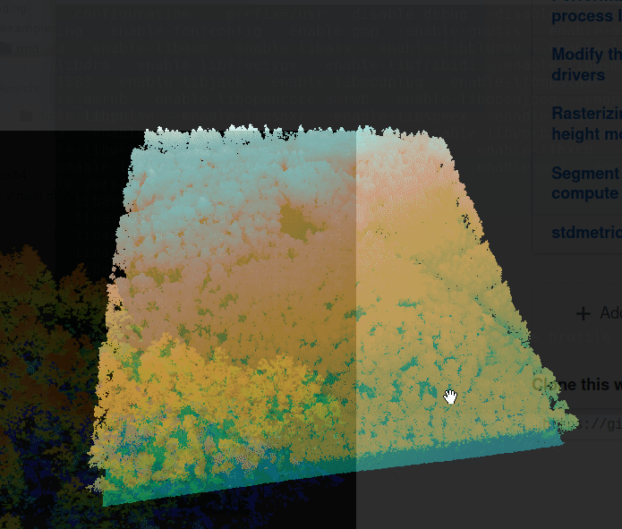
The whole clipped MOF area rendered to a canopy height model.
Full screen version of the map
Assuming this script (or the script you have adapted) runs without any technical errors, the exciting part of the data preprocessing comes now:
- which algorithms did I use and why?
- 45m high trees - does that make sense?
- if not why not? What happens and correction options do I have? Is the error due to the data, the algorithms, the script or all together?
Where to go?
To answer this questions we need a two folded approach. First we need technically to strip down the script to a real control script, all functionality that is used more than once will be moved into functions or other static scripts. Second in a more applied or scientific way we need to find out what algorithm is most suitable and reliable to answer our questions.
- Technically everything is prepared to dive into tree segmentation strategies.