## ##
# ---- 0 Projekt Setup ----
require("pacman")
#remotes::install_github("zivankaraman/CDSE")
# packages installing if necessary and loading
pacman::p_load(mapview, mapedit, tmap, tmaptools, raster, terra, stars, gdalcubes, sf, dplyr,CDSE, downloader, tidyverse,RStoolbox,rprojroot, exactextractr, randomForest, ranger, e1071, caret, link2GI, rstac, OpenStreetMap,colorspace)

#--- Switch to determine whether digitization is required. If set to FALSE, the
root_folder = find_rstudio_root_file()

m1 = tm_shape(pred_stack_2019) + tm_rgb(r=4, g=3, b=2) +
  tm_layout(legend.outside.position = "right",
            legend.outside = T,
            panel.label.height=0.6,
            panel.label.size=0.6,
            panel.labels = c("r=1, g=2, b=3")) +
  tm_grid()

m2 = tm_shape(pred_stack_2019) + tm_rgb(r=8, g=4, b=3) +
  tm_layout(legend.outside.position = "right",
            legend.outside = T,
            panel.label.height=0.6,
            panel.label.size=0.6,
            panel.labels = c("r=8, g=4, b=3")) +
  tm_grid()
tmap::tmap_arrange(m1,m2)Untitled
Creating training areas with mapedit
With mapedit, each class must be digitized individually. Once the training areas are available as vector data, the features of the respective raster stack can be extracted into a table according to the digitized classes and corrected for possible missing values.
Using color composites for better training results
For this exercise, we use mapedit, a small but powerful package that allows you to digitize and edit vector data in Rstudio or an external browser. In combination with mapview, any [color composite] (https://custom-scripts.sentinel-hub.com/custom-scripts/sentinel-2/composites/) can also be used as a basis for digitization.
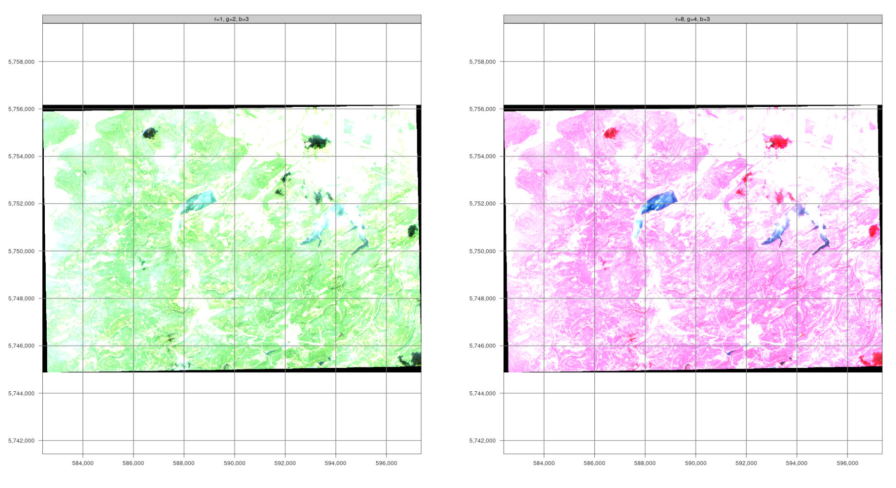
The planes can be switched using the plane control. In true-color composites, the visible spectral channels Red (B04), Green (B03), and Blue (B02) are mapped to the corresponding red, green, and blue color channels, respectively, producing an image of the surface that closely resembles the natural “color” as it would be seen by a human sitting on the spacecraft. False color images are often created using the spectral channels for near-infrared, red, and green. They are particularly useful for assessing vegetation because plants reflect near-infrared and green light while absorbing red light (red-edge effect). Dense vegetation appears a darker red. Cities and open ground appear gray or light brown, water appears blue or black.
## ##

#---- Digitization of training data ----

if (digitize) {
# For the supervised classification, we need training areas. You can digitize them as shown below or alternatively use QGis, for example

# clearcut

# For the false color composite r = 8, g = 4, b = 3, maxpixels = 1693870)
# maxpixels has significantly higher memory requirements, vegetation in red
# below the true color composite
train_area_2019 <- mapview::viewRGB(pred_stack_2019, r = 4, g = 3, b = 2, maxpixels = 1693870) %>% mapedit::editMap()
# Adding the attributes class (text) and id/year (integer)
clearcut_2019 <- train_area_2019$finished$geometry %>% st_sf() %>% mutate(class = "clearcut", id = 1,year=2019)
train_area_2020 <- mapview::viewRGB(pred_stack_2020, r = 4, g = 3, b = 2,maxpixels = 1693870) %>% mapedit::editMap()
clearcut_2020 <- train_area_2020$finished$geometry %>% st_sf() %>% mutate(class = "clearcut", id = 1,year=2020)

# other: all areas not belonging to clear cutting as representative as possible
train_area_2019 <- mapview::viewRGB(pred_stack_2019, r = 4, g = 3, b = 2) %>% mapedit::editMap()
other_2019 <- train_area_2019$finished$geometry %>% st_sf() %>% mutate(class = "other", id = 2,year=2019)
train_area_2020 <- mapview::viewRGB(pred_stack_2020, r = 4, g = 3, b = 2) %>% mapedit::editMap()
other_2020 <- train_area_2020$finished$geometry %>% st_sf() %>% mutate(class = "other", id = 2,year=2020)

train_areas_2019_2020 <- rbind(clearcut_2019,clearcut_2020, other_2019,other_2020) # Reproject to the raster file
train_areas_2019 = sf::st_transform(train_areas_2019_2020,crs = sf::st_crs(pred_stack_2019))
mapview(filter(train_areas_2019_2020,year==2019), zcol="class")
# save geometries
st_write(train_areas_2019_2020,paste0(envrmt$path_data,"train_areas_2019_2020.gpkg"))

# Extract the training data for the digitized areas
tDF_2019 = exactextractr::exact_extract(pred_stack_2019, filter(train_areas_2019_2020,year==2019), force_df = TRUE,
include_cell = TRUE,include_xy = TRUE,full_colnames = TRUE,include_cols = "class")
tDF_2020 = exactextractr::exact_extract(pred_stack_2020, filter(train_areas_2019_2020,year==2020), force_df = TRUE,
include_cell = TRUE,include_xy = TRUE,full_colnames = TRUE,include_cols = "class")

# again, copy together into a file
tDF_2019 = dplyr::bind_rows(tDF_2019)
tDF_2019$year = 2019
tDF_2020 = dplyr::bind_rows(tDF_2020)
tDF_2020$year = 2020
# Delete any rows that contain NA (no data) values
tDF_2019 = tDF_2019[complete.cases(tDF_2019) ,]
tDF_2020 = tDF_2020[complete.cases(tDF_2020) ,]

tDF= rbind(tDF_2019,tDF_2020)

# check the extracted data
summary(tDF)

# Save as R internal data format
# is stored in the repo and can therefore be loaded (line below)
saveRDS(tDF, paste0(envrmt$path_data,"tDF.rds"))


} else {
tDF = readRDS(paste0(envrmt$path_data,"tDF.rds"))
}
The result is a table with training data for 2019 and 2020. The data set contains all raster information for all bands covered by the polygons for the classes “clearcut” and “other”.
## ##
head(tDF)