#------------------------------------------------------------------------------
# Author: creuden@gmail.com
# Description:  cleans climate data from ecowitt stations and interpolates the air temp
# Copyright:GPL (>= 3)  Date: 2024-09-28
#------------------------------------------------------------------------------

# 0 ---- project setup ----

# load packages (if not installed please install via install.packages())
require("pacman")
# packages installing if necessary and loading
pacman::p_load(mapview, mapedit, tmap, tmaptools, raster, terra, stars, gdalcubes,
               sf,webshot, dplyr,CDSE,webshot, downloader, tidyverse,RStoolbox,
               rprojroot, exactextractr, randomForest, ranger, e1071, caret,
               link2GI, rstac, OpenStreetMap,colorspace,ows4R,httr,
               lwgeom,readxl,highfrequency,tibble,xts,data.table,gstat)

# create a string containing the current working directory
wd=paste0(find_rstudio_root_file(),"/data/")

# define time period to aggregate temp data in hours
time_period = 3

# multiplication factor for blowing up the Copernicus DEM
blow_fac = 15

# reference system as proj4 string for old SP package related stuff
crs = raster::crs("+proj=utm +zone=33 +datum=WGS84 +units=m +no_defs")
sfcrs <- st_crs("EPSG:32633")

# Copernicus DEM (https://land.copernicus.eu/imagery-in-situ/eu-dem/eu-dem-v1.1)
fnDTM = paste0(wd,"copernicus_DEM.tif")

# Weather Data adapt if you download a new file
# https://www.ecowitt.net/home/index?id=20166)
# https://www.ecowitt.net/home/index?id=149300
fn_dataFC29 = paste0(wd,"all_GW1000A-WIFIFC29.xlsx")
fn_dataDB2F =paste0(wd,"all_GW1000A-WIFIDB2F.xlsx")

# station data as derived by the field group
fn_pos_data= paste0(wd,"stations_prelim.shp")

# arbitrary plot borders just digitized for getting a limiting border of the plot area
fn_area =paste0(wd,"plot.shp")

# rds file for saving the cleaned up weather data
cleandata = paste0(wd,"climdata.RDS")
# end setupSpatial Interpolation - Harz Summerschool Example
Example air temperature - Microclimate
The following example shows a typical practical application. As part of the EON Summerschool, field and remote sensing methods as well as methods of data collection and evaluation are taught using practical examples. In this context, climate stations have been repeatedly used in different areas, especially in deadwood and clear-cut areas. Since these are only point measurements, the question naturally arises as to how the temperature and humidity values are distributed spatially and how they can be predicted using drone data, for example. In addition to the handling of the stations, the raw data from the CSV/Excel tables must of course first be cleaned up, which involves a considerable amount of work with Ecowitt’s data formats. In a second step, simple interpolation methods will be demonstrated.
Setup of the project
Data preprocessing and cleaning
# 1 ---- preprocessing ----
# read_sf("data/de_nuts1.gpkg") |> st_transform(crs) -> de
# read DEM data
DTM = terra::rast(fnDTM) # DTM.
# increase resolution by 15
DTM=disagg(DTM, fact=c(blow_fac, blow_fac))
#rename layer to altitude
names(DTM)="altitude"
r=DTM*0

# read station position data
pos=st_read(fn_pos_data)
Reading layer `stations_prelim' from data source
`/home/creu/edu/gisma-courses/LV-19-d19-006-24/reader/data/stations_prelim.shp'
using driver `ESRI Shapefile'
Simple feature collection with 14 features and 1 field
Geometry type: POINT
Dimension: XY
Bounding box: xmin: 183055.8 ymin: 5748366 xmax: 183170.3 ymax: 5748499
Projected CRS: WGS 84 / UTM zone 33N# read station position data
area=st_read(fn_area)Reading layer `plot' from data source
`/home/creu/edu/gisma-courses/LV-19-d19-006-24/reader/data/plot.shp'
using driver `ESRI Shapefile'
Simple feature collection with 1 feature and 1 field
Geometry type: POLYGON
Dimension: XY
Bounding box: xmin: 10.40154 ymin: 51.79506 xmax: 10.40658 ymax: 51.79803
Geodetic CRS: WGS 84# reproject the dataset to the project crs
area=st_transform(area,crs)
# read temperature data we need to skip row 1 due to excel format
clim_dataFC29 = as_tibble(readxl::read_excel(fn_dataFC29, skip = 1)) New names:
• `` -> `...1`
• `Temperature(℃)` -> `Temperature(℃)...2`
• `Temperature Low(℃)` -> `Temperature Low(℃)...3`
• `Temperature High(℃)` -> `Temperature High(℃)...4`
• `Humidity(%)` -> `Humidity(%)...7`
• `Humidity Low(%)` -> `Humidity Low(%)...8`
• `Humidity High(%)` -> `Humidity High(%)...9`
• `Temperature(℃)` -> `Temperature(℃)...10`
• `Temperature Low(℃)` -> `Temperature Low(℃)...11`
• `Temperature High(℃)` -> `Temperature High(℃)...12`
• `Humidity(%)` -> `Humidity(%)...13`
• `Humidity Low(%)` -> `Humidity Low(%)...14`
• `Humidity High(%)` -> `Humidity High(%)...15`
• `Temperature(℃)` -> `Temperature(℃)...32`
• `Temperature Low(℃)` -> `Temperature Low(℃)...33`
• `Temperature High(℃)` -> `Temperature High(℃)...34`
• `Humidity(%)` -> `Humidity(%)...35`
• `Temperature(℃)` -> `Temperature(℃)...36`
• `Temperature Low(℃)` -> `Temperature Low(℃)...37`
• `Temperature High(℃)` -> `Temperature High(℃)...38`
• `Humidity(%)` -> `Humidity(%)...39`
• `Temperature(℃)` -> `Temperature(℃)...40`
• `Temperature Low(℃)` -> `Temperature Low(℃)...41`
• `Temperature High(℃)` -> `Temperature High(℃)...42`
• `Humidity(%)` -> `Humidity(%)...43`
• `Temperature(℃)` -> `Temperature(℃)...44`
• `Temperature Low(℃)` -> `Temperature Low(℃)...45`
• `Temperature High(℃)` -> `Temperature High(℃)...46`
• `Humidity(%)` -> `Humidity(%)...47`
• `Temperature(℃)` -> `Temperature(℃)...48`
• `Temperature Low(℃)` -> `Temperature Low(℃)...49`
• `Temperature High(℃)` -> `Temperature High(℃)...50`
• `Humidity(%)` -> `Humidity(%)...51`
• `Temperature(℃)` -> `Temperature(℃)...52`
• `Temperature Low(℃)` -> `Temperature Low(℃)...53`
• `Temperature High(℃)` -> `Temperature High(℃)...54`
• `Humidity(%)` -> `Humidity(%)...55`
• `Temperature(℃)` -> `Temperature(℃)...56`
• `Temperature Low(℃)` -> `Temperature Low(℃)...57`
• `Temperature High(℃)` -> `Temperature High(℃)...58`
• `Humidity(%)` -> `Humidity(%)...59`
• `Temperature(℃)` -> `Temperature(℃)...60`
• `Temperature Low(℃)` -> `Temperature Low(℃)...61`
• `Temperature High(℃)` -> `Temperature High(℃)...62`
• `Humidity(%)` -> `Humidity(%)...63`
• `Soilmoisture(%)` -> `Soilmoisture(%)...64`
• `Soilmoisture(%)` -> `Soilmoisture(%)...65`
• `Soilmoisture(%)` -> `Soilmoisture(%)...66`
• `Soilmoisture(%)` -> `Soilmoisture(%)...67`
• `Soilmoisture(%)` -> `Soilmoisture(%)...68`
• `Soilmoisture(%)` -> `Soilmoisture(%)...69`
• `Soilmoisture(%)` -> `Soilmoisture(%)...70`
• `Soilmoisture(%)` -> `Soilmoisture(%)...71`clim_dataDB2F = as_tibble(readxl::read_excel(fn_dataDB2F, skip = 1))New names:
• `` -> `...1`
• `Temperature(℃)` -> `Temperature(℃)...2`
• `Temperature Low(℃)` -> `Temperature Low(℃)...3`
• `Temperature High(℃)` -> `Temperature High(℃)...4`
• `Humidity(%)` -> `Humidity(%)...7`
• `Humidity Low(%)` -> `Humidity Low(%)...8`
• `Humidity High(%)` -> `Humidity High(%)...9`
• `Temperature(℃)` -> `Temperature(℃)...10`
• `Temperature Low(℃)` -> `Temperature Low(℃)...11`
• `Temperature High(℃)` -> `Temperature High(℃)...12`
• `Humidity(%)` -> `Humidity(%)...13`
• `Humidity Low(%)` -> `Humidity Low(%)...14`
• `Humidity High(%)` -> `Humidity High(%)...15`
• `Temperature(℃)` -> `Temperature(℃)...25`
• `Temperature Low(℃)` -> `Temperature Low(℃)...26`
• `Temperature High(℃)` -> `Temperature High(℃)...27`
• `Humidity(%)` -> `Humidity(%)...28`
• `Temperature(℃)` -> `Temperature(℃)...29`
• `Temperature Low(℃)` -> `Temperature Low(℃)...30`
• `Temperature High(℃)` -> `Temperature High(℃)...31`
• `Humidity(%)` -> `Humidity(%)...32`
• `Temperature(℃)` -> `Temperature(℃)...33`
• `Temperature Low(℃)` -> `Temperature Low(℃)...34`
• `Temperature High(℃)` -> `Temperature High(℃)...35`
• `Humidity(%)` -> `Humidity(%)...36`
• `Temperature(℃)` -> `Temperature(℃)...37`
• `Temperature Low(℃)` -> `Temperature Low(℃)...38`
• `Temperature High(℃)` -> `Temperature High(℃)...39`
• `Humidity(%)` -> `Humidity(%)...40`
• `Temperature(℃)` -> `Temperature(℃)...41`
• `Temperature Low(℃)` -> `Temperature Low(℃)...42`
• `Temperature High(℃)` -> `Temperature High(℃)...43`
• `Humidity(%)` -> `Humidity(%)...44`
• `Temperature(℃)` -> `Temperature(℃)...45`
• `Temperature Low(℃)` -> `Temperature Low(℃)...46`
• `Temperature High(℃)` -> `Temperature High(℃)...47`
• `Humidity(%)` -> `Humidity(%)...48`
• `Temperature(℃)` -> `Temperature(℃)...49`
• `Temperature Low(℃)` -> `Temperature Low(℃)...50`
• `Temperature High(℃)` -> `Temperature High(℃)...51`
• `Humidity(%)` -> `Humidity(%)...52`
• `Temperature(℃)` -> `Temperature(℃)...53`
• `Temperature Low(℃)` -> `Temperature Low(℃)...54`
• `Temperature High(℃)` -> `Temperature High(℃)...55`
• `Humidity(%)` -> `Humidity(%)...56`# select the required cols
tempFC29 = clim_dataFC29 %>% dplyr::select(c(1,2,32,36,40,44,48))
tempDB2F = clim_dataDB2F %>% dplyr::select(c(1,25,29,33,37,41,45,49,53))
# rename header according to the pos file names and create a merge field time
names(tempDB2F) = c("time","ch1_r","ch2_r","ch3_r","ch4_r","ch5_r","ch6_r","ch7_r","ch8_r")
names(tempFC29) = c("time","base","ch1","ch2","ch3","ch4","ch5")
#merge files
temp=merge(tempFC29,tempDB2F)
# convert datum which is a string to date format
temp$time=as.POSIXct(temp$time)
# aggregate timeslots according to the value in time_period
temp3h = highfrequency::aggregateTS(xts::as.xts(temp), alignBy = "hours",dropna = T,alignPeriod = time_period)
# add the datum colum (which is now a pointer of the timeseries) as first col in the dataset
temp_fin=as_tibble(temp3h) %>% add_column(time = zoo::index(temp3h), .before = 1)
# transpose and combine the table
temp_fin=as_tibble(cbind(nms = names(temp_fin), t(temp_fin)))Warning: The `x` argument of `as_tibble.matrix()` must have unique column names if
`.name_repair` is omitted as of tibble 2.0.0.
ℹ Using compatibility `.name_repair`.# delete first row
names(temp_fin) = temp_fin[1,]Warning: The `value` argument of `names<-()` must be a character vector as of tibble
3.0.0.temp_fin=temp_fin[-1,]
# replace names specially time by stationid
names(temp_fin)[names(temp_fin) == 'time'] = 'stationid'
# extract altitudes for positions
pos$altitude= exactextractr::exact_extract(DTM,st_buffer(pos,1),"mean")
  |
  |                                                                      |   0%
  |
  |=====                                                                 |   7%
  |
  |==========                                                            |  14%
  |
  |===============                                                       |  21%
  |
  |====================                                                  |  29%
  |
  |=========================                                             |  36%
  |
  |==============================                                        |  43%
  |
  |===================================                                   |  50%
  |
  |========================================                              |  57%
  |
  |=============================================                         |  64%
  |
  |==================================================                    |  71%
  |
  |=======================================================               |  79%
  |
  |============================================================          |  86%
  |
  |=================================================================     |  93%
  |
  |======================================================================| 100%
# merge positions and values via id
m=merge(pos,temp_fin)
# make the var name working for gstat by replacing all patterns
n= gsub(x = names(m),pattern = "-",replacement = "")
n= gsub(x = n,pattern = " ",replacement = "")
n= gsub(x = n,pattern = ":",replacement = "")
n= gsub(x = n,pattern = "2023",replacement = "A2023")
# and rename couse this as new names
names(m)=n
m= st_transform(m,sfcrs)
saveRDS(m,cleandata)
# grep the varnames for an interpolation loop
vars=grep(glob2rx("A2023*"), n, value = TRUE)
vars[1] "A20230828230000" "A20230829020000" "A20230829050000" "A20230829080000"
[5] "A20230829110000" "A20230829140000" "A20230829170000" "A20230829200000"
[9] "A20230829220000"# convert final sf vector to terra vector
temperature_vect = vect(m)
temperature_vect class : SpatVector
geometry : points
dimensions : 14, 11 (geometries, attributes)
extent : 183055.8, 183170.3, 5748366, 5748499 (xmin, xmax, ymin, ymax)
coord. ref. : WGS 84 / UTM zone 33N (EPSG:32633)
names : stationid altitude A20230828230000 A20230829020000
type : <chr> <num> <chr> <chr>
values : base 579.1 10.3 10.1
ch1 578 10.6 10.2
ch1_r 575.3 10.7 10.0
A20230829050000 A20230829080000 A20230829110000 A20230829140000
<chr> <chr> <chr> <chr>
9.5 9.6 14.8 13
9.5 9.7 12 14.3
9.6 10.4 13.4 18.3
A20230829170000 A20230829200000 A20230829220000
<chr> <chr> <chr>
15.2 12.8 11.5
16.9 12.9 10.4
19.2 9.9 8.1# create table containing x, y, value (A20230829220000) to interpolate this values in space
xyz=cbind(geom(temperature_vect)[,3],geom(temperature_vect)[,4],as.numeric(temperature_vect$A20230829220000))
# convert to data frame and name header
xyz=data.frame(xyz)
names(xyz) =c("x","y","temp")
xyz x y temp
1 183137.7 5748385 11.5
2 183087.0 5748438 10.4
3 183130.3 5748437 8.1
4 183055.8 5748460 10.7
5 183098.0 5748374 9.7
6 183081.0 5748499 10.6
7 183110.5 5748389 9.7
8 183095.5 5748465 10.7
9 183144.5 5748366 8.9
10 183120.1 5748476 10.5
11 183170.3 5748415 6.4
12 183144.8 5748427 7.4
13 183156.8 5748389 7.4
14 183134.0 5748399 7.8# the same just for x,y
xy=cbind(geom(temperature_vect)[,3],geom(temperature_vect)[,4])
#the same just for z
z=as.numeric(temperature_vect$A20230829220000)
# end of preprocessingInterpolation approaches
# 2 ---- interpolation ----

# -terra package
# 2.1 ---- Voronoi Segmentation ----
p = vect(xyz, geom=c("x", "y"))
voronoi = voronoi(p)
v = sf::st_as_sf(p)
sf::st_crs(v)= sfcrs


# 2.2 ---- Nearest neighbor interpolation ----
interpNN = interpNear(r, as.matrix(xyz),radius=100)

# 2.3 ----  Inverse Distance interpolation ----
interpIDW = interpIDW(r, as.matrix(xyz), radius=300, power=2, smooth=1, maxPoints=3)
# ploting
plot(interpIDW)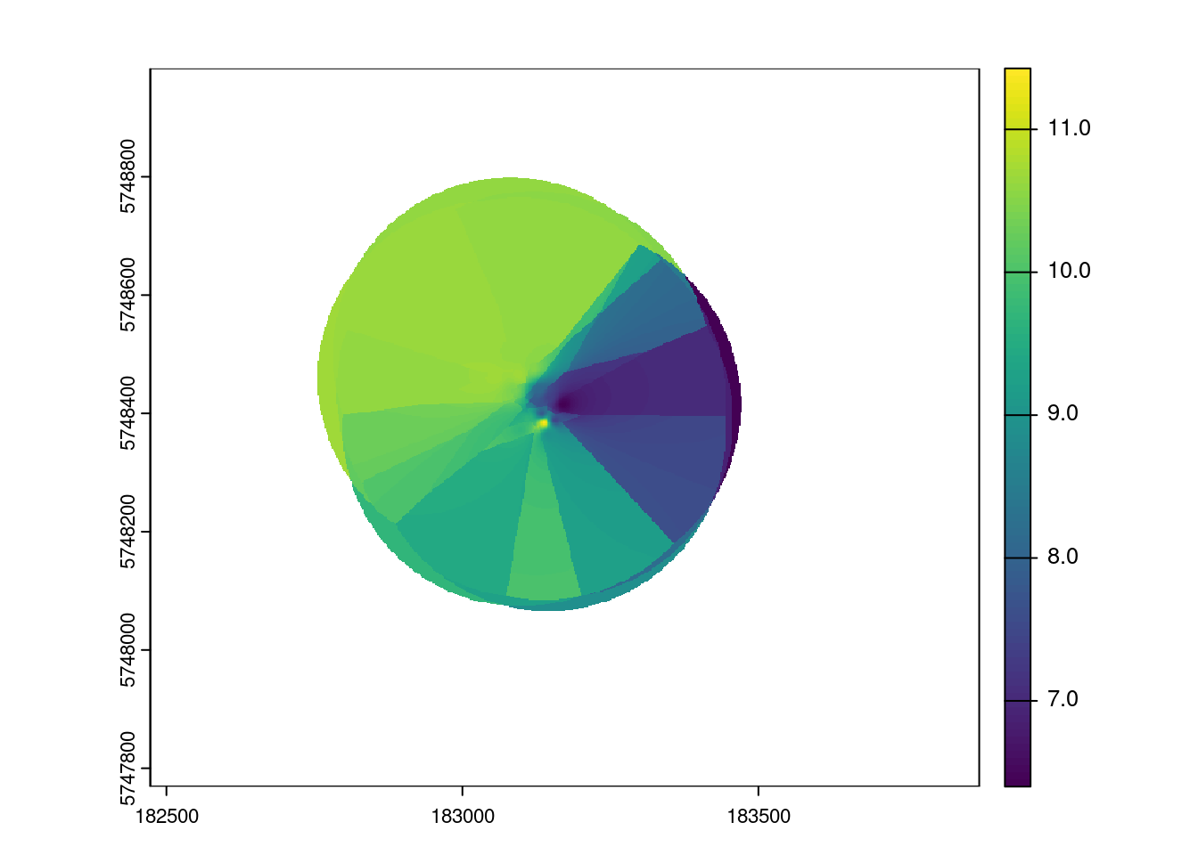
# 2.4  ---- utilizing the gstat package Inverse Distance interpolation ----
idw_gstat <- gstat::idw(A20230829220000~1, m, st_as_stars(r),nmin = 3, maxdist = 100, idp = 2.0)
[inverse distance weighted interpolation]# ploting
plot(idw_gstat)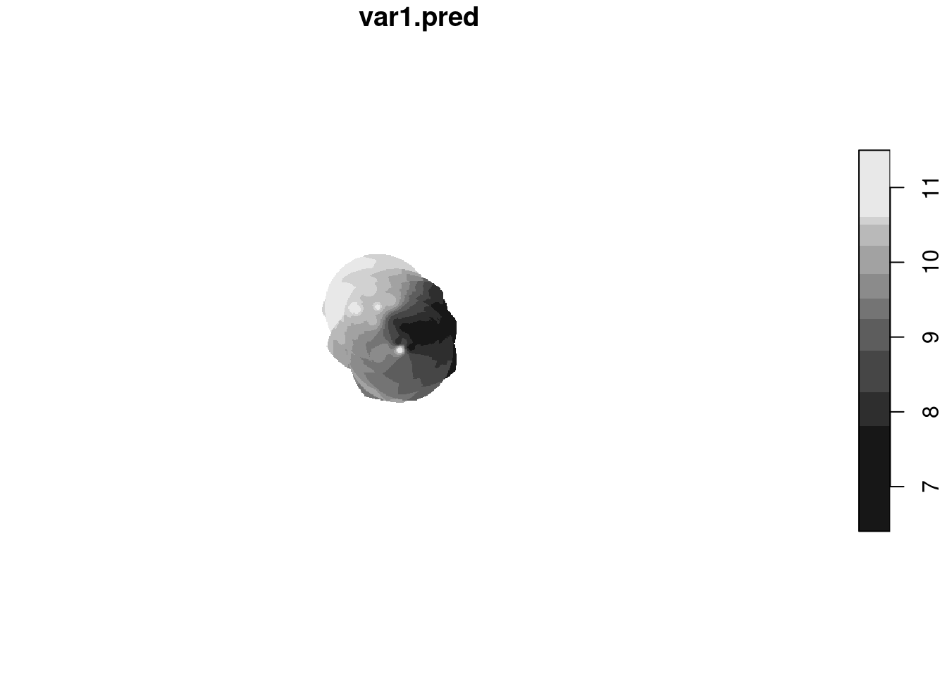
# 2.4 ---- utilizing the gstat package kriging
# first convert terra spatraster to stars and set name to altitude
dtm = setNames(st_as_stars(DTM),"altitude")
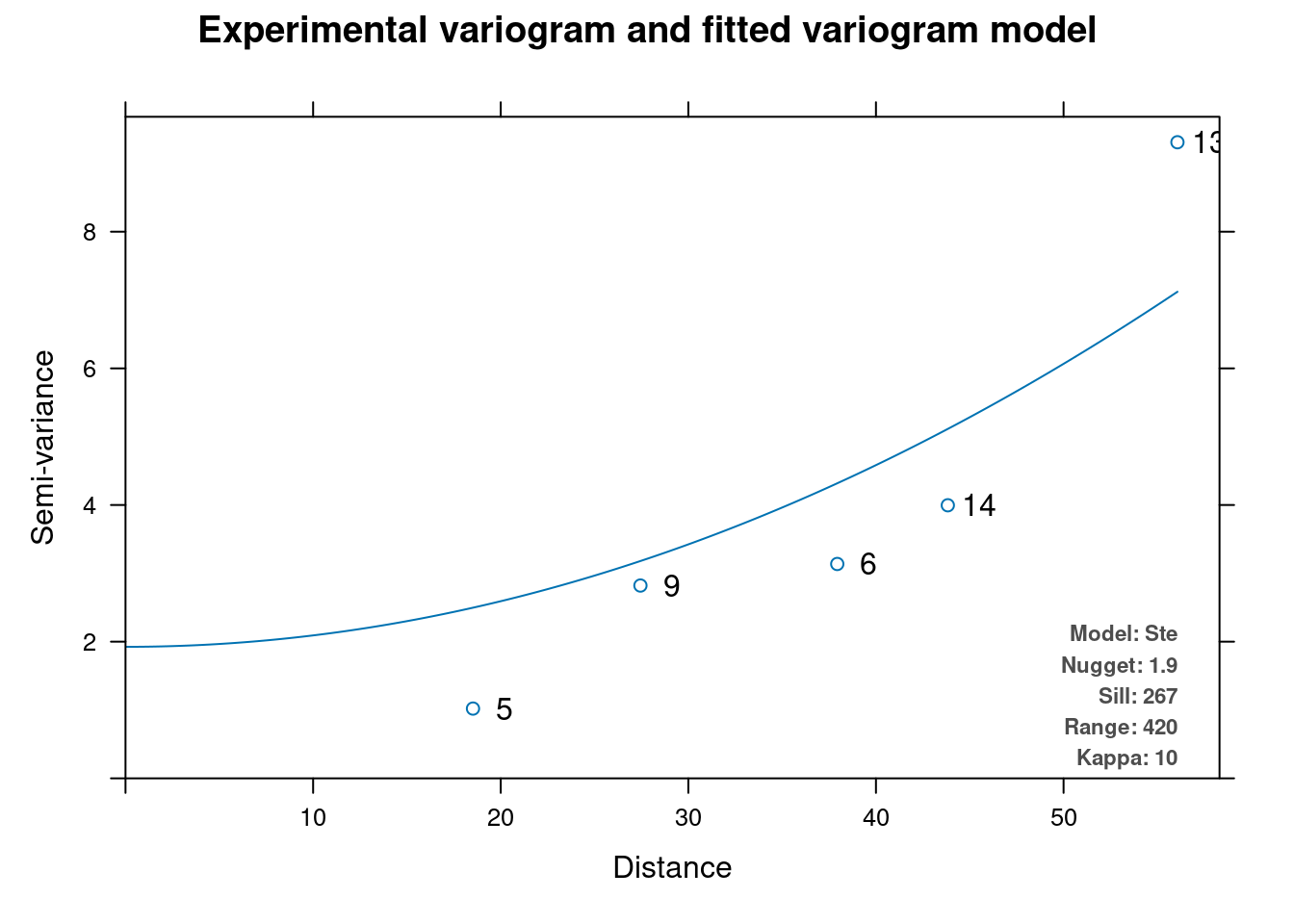
# create an autovariogram model
vm.auto = automap::autofitVariogram(formula = as.formula(paste("altitude", "~ 1")),
input_data = m)
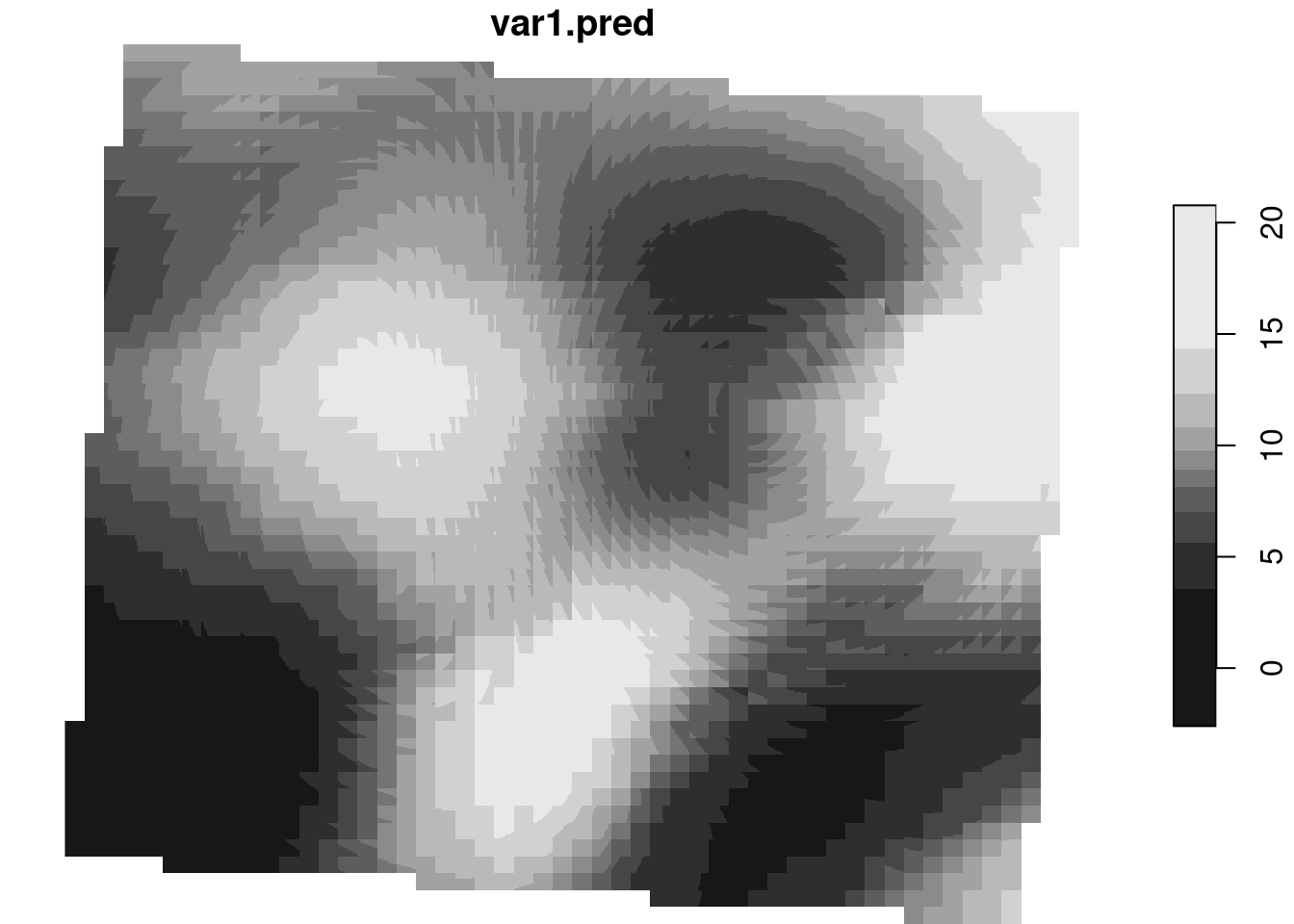
k <- krige(A20230829220000 ~ altitude, m, dtm,
vm.auto$var_model)[using universal kriging]plot(k)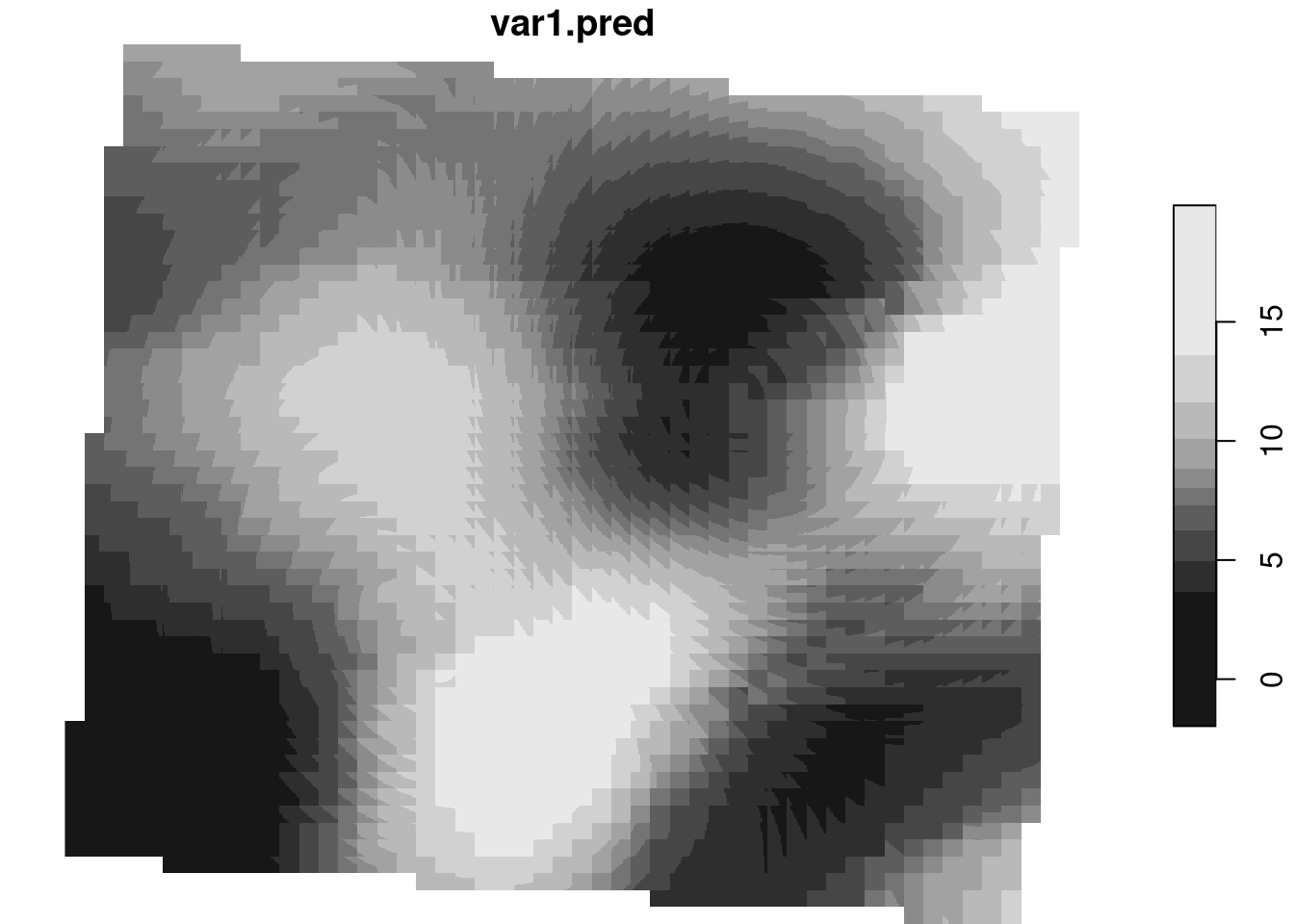
# map it
mapview(raster(interpNN) ,col=rainbow(25)) +
  mapview( raster(interpIDW),col=rainbow(25)) +
  mapview(k,col=rainbow(25))+ v
Warning in rasterCheckSize(x, maxpixels = maxpixels): maximum number of pixels for Raster* viewing is 5e+05 ;
the supplied Raster* has 608400
... decreasing Raster* resolution to 5e+05 pixels
to view full resolution set 'maxpixels = 608400 '
Warning in rasterCheckSize(x, maxpixels = maxpixels): maximum number of pixels for Raster* viewing is 5e+05 ;
the supplied Raster* has 608400
... decreasing Raster* resolution to 5e+05 pixels
to view full resolution set 'maxpixels = 608400 'Number of pixels is above 5e+05. Automatic downsampling of `stars` object is not yet implemented, so rendering may be slow.
You can pass a `stars` proxy object to mapview to get automatic downsampling.## universal kriging with gstat
# we use the terrain model for prediction
# for all time slots
for (var in vars[7:8]){
# autofit variogramm for kriging
vm.auto = automap::autofitVariogram(formula = as.formula(paste("altitude", "~ 1")),
input_data = m)
plot(vm.auto)
# # kriging
print(paste0("kriging ", var))
k <- gstat::krige( as.formula(paste(var, " ~ altitude")), m, dtm,
vm.auto$var_model)
plot(k)
# save to geotiff
stars::write_stars(k,paste0(wd,var,"v_interpol.tif"),overwrite=TRUE)
}
[1] "kriging A20230829170000"
[using universal kriging]
Warning in write_stars.stars(k, paste0(wd, var, "v_interpol.tif"), overwrite =
TRUE): all but first attribute are ignored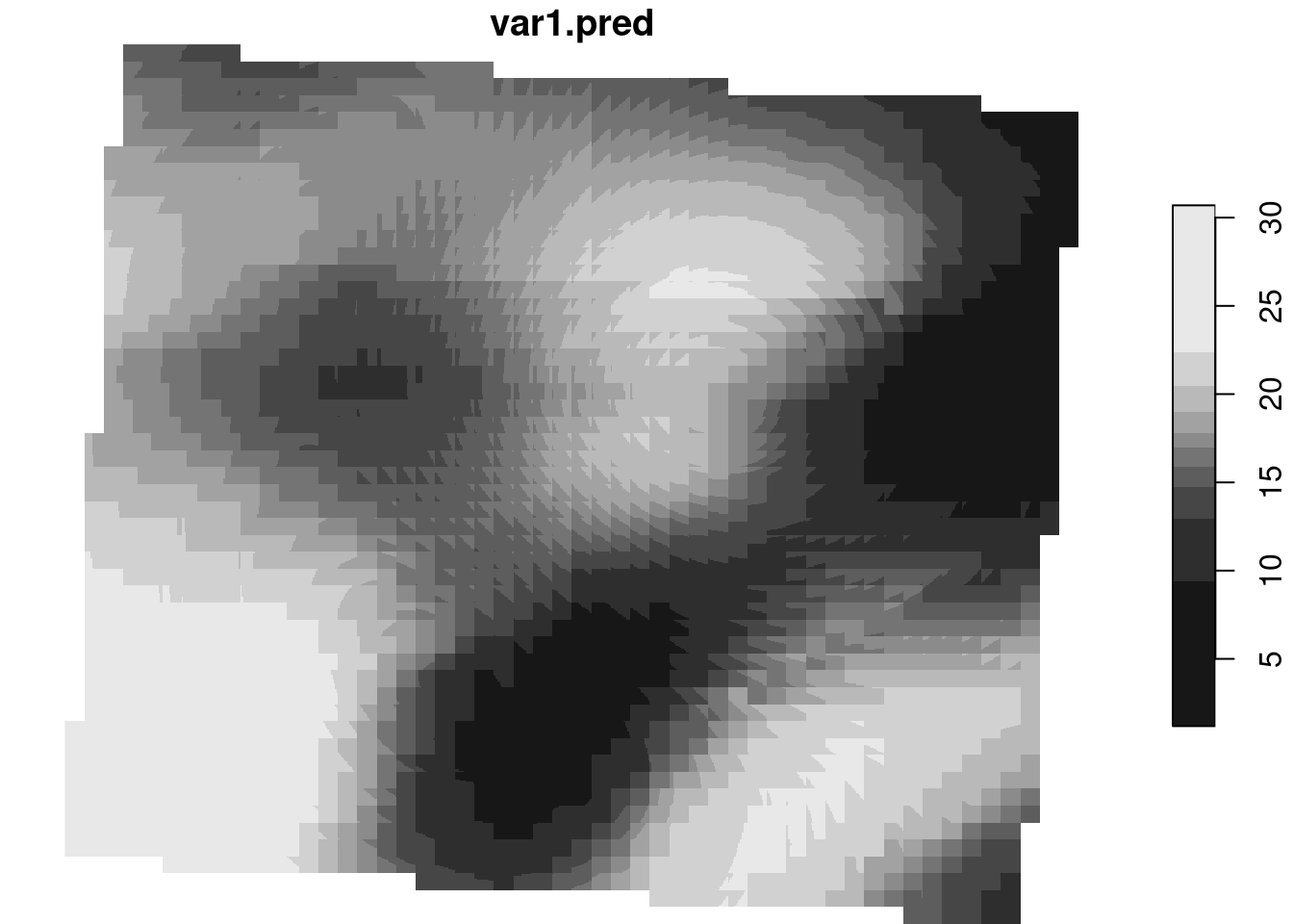
[1] "kriging A20230829200000"
[using universal kriging]
Warning in write_stars.stars(k, paste0(wd, var, "v_interpol.tif"), overwrite =
TRUE): all but first attribute are ignored